CENFA provides tools for performing ecological-niche
factor analysis (ENFA) and climate-niche factor analysis (CNFA). This
package was created with three goals in mind:
CENFA takes advantage of the raster and
sp packages, allowing the user to conduct analyses directly
with raster, shapefile, and point data, and to handle large datasets
efficiently via partial data loading and parallelization.
You can install the most recent version of CENFA from GitHub with:
# install.packages("devtools")
devtools::install_github("rinnan/CENFA")enfaWe will use some example datasets to perform a basic ENFA. The
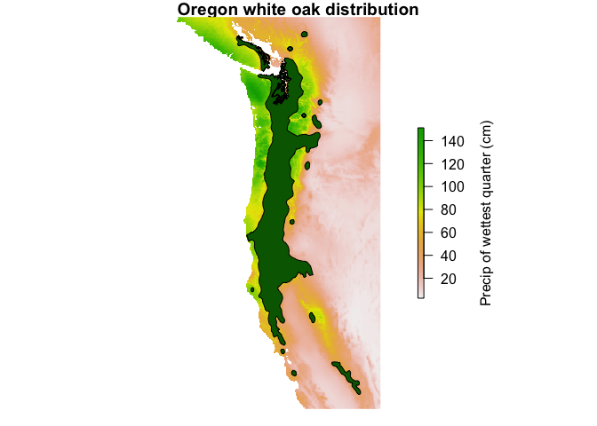
historical climate dataset climdat.hist is a RasterBrick of
10 climate variables, covering much of the western US coast.
QUGA is a SpatialPolygonsDataFrame of the historical range
map of Oregon white oak (Quercus garryana).
A plot of the data, using the one of the layers of
climdat.hist:
The enfa function takes three basic arguments: the
dataset of ecological variables (climdat.hist), the map of
species presence (QUGA), and the values of
QUGA that specify presence (in this case, a column named
“CODE”). Calling the enfa object by name provides a
standard summary of the ENFA results.
mod.enfa <- enfa(x = climdat.hist, s.dat = QUGA, field = "CODE")
mod.enfa
#> ENFA
#>
#> Original function call: enfa(x = climdat.hist, s.dat = QUGA, field = "CODE")
#>
#> Marginality factor:
#>   MDR   ISO    TS HMmax CMmin   PWM   PDM    PS   PWQ   PDQ
#> -0.13  0.51 -0.67 -0.03  0.67  0.71 -0.13  0.70  0.72  0.13
#>
#> Eigenvalues of specialization:
#>  Marg Spec1 Spec2 Spec3 Spec4 Spec5 Spec6 Spec7 Spec8 Spec9
#>  5.12  8.92  4.82  3.01  2.55  2.01  1.28  0.77  0.68  0.36
#>
#> Percentage of specialization contained in ENFA factors:
#>  Marg Spec1 Spec2 Spec3 Spec4 Spec5 Spec6 Spec7 Spec8 Spec9
#> 17.36 30.24 16.32 10.20  8.64  6.80  4.33  2.61  2.30  1.21
#>
#> Overall marginality:  1.654
#>
#> Overall specialization:  1.718
#>
#> Significant ENFA factors:
#>        Marg Spec1 Spec2 Spec3
#> MDR   -0.13 -0.46  0.59  0.38
#> ISO    0.51  0.11 -0.46 -0.05
#> TS    -0.67 -0.34 -0.54  0.39
#> HMmax -0.03  0.58 -0.07 -0.57
#> CMmin  0.67 -0.54  0.00  0.49
#> PWM    0.71 -0.08  0.26  0.27
#> PDM   -0.13  0.10  0.09  0.03
#> PS     0.70  0.12 -0.11 -0.02
#> PWQ    0.72  0.03 -0.19 -0.25
#> PDQ 0.13 0.00 -0.11 -0.04scatterWe can visualize the ENFA results via the scatter
function, which produces a biplot of the marginality axis and one of the
specialization axes. This gives us a portrait of the species’ niche to
compare with the global niche of the reference study area, with the
ecological axes projected onto the ENFA dimensions. (Note: since
mod.enfa only contains information about the species
habitat, we must first construct a GLcenfa object that also
describes the global habitat.)
glc <- GLcenfa(x = climdat.hist)
scatter(x = mod.enfa, y = glc)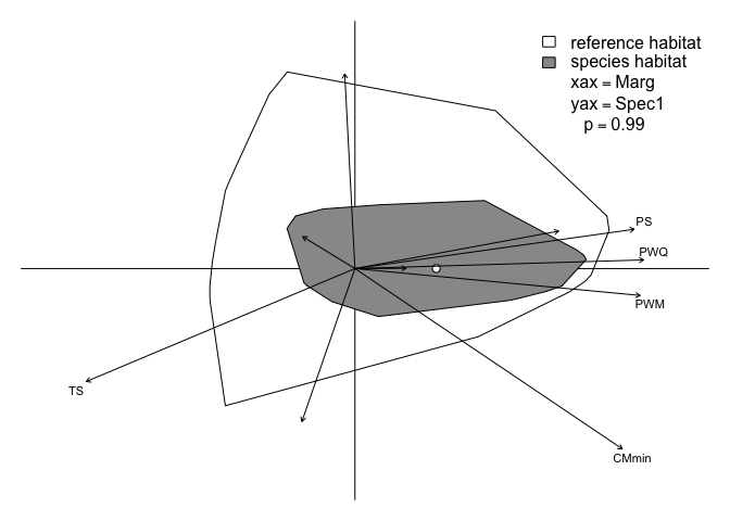
For larger datasets, we can speed up the computation via
parallelization. We provide two additional arguments,
parallel = TRUE, and n, which specifies the
number of cores to use. n has a default value of 1, so only
setting parallel = TRUE will not parallelize the function
by itself.
# does not enable parallelization
mod <- enfa(x = climdat.hist, s.dat = QUGA, field = "CODE", parallel = TRUE)

# enables parallelization across 4 cores
mod <- enfa(x = climdat.hist, s.dat = QUGA, field = "CODE", parallel = TRUE, n = 4)
The function will attempt to match the value provided to
n with the number of cores detected on the local device via
parallel::detectCores(); if the provided n is
greater than the number of available cores k, a warning
will be issued and n will be set to k - 1.
cnfaThe cnfa function is very similar to enfa,
but performs a slightly different analysis. Whereas ENFA returns a
specialization factor (the eigenvalues of specialization)
describing the amount of specialization found in each ENFA
factor, CNFA returns a sensitivity factor that reflects
the amount of sensitivity found in each ecological variable.
This makes the sensitivity factor more directly comparable to the
marginality factor, and more interpretable in the context of species’
sensitivity to a given variable.
mod.cnfa <- cnfa(x = climdat.hist, s.dat = QUGA, field = "CODE")
mod.cnfa
#> CNFA
#>
#> Original function call: cnfa(x = climdat.hist, s.dat = QUGA, field = "CODE")
#>
#> Marginality factor:
#>   MDR   ISO    TS HMmax CMmin   PWM   PDM    PS   PWQ   PDQ
#> -0.13  0.51 -0.67 -0.03  0.67  0.71 -0.13  0.70  0.72  0.13
#>
#> Sensitivity factor:
#>   MDR   ISO    TS HMmax CMmin   PWM   PDM    PS   PWQ   PDQ
#>  4.52  2.86  4.16  3.72  3.98  3.36  1.35  1.71  2.94  0.92
#>
#> Percentage of specialization contained in CNFA factors:
#>  Marg Spec1 Spec2 Spec3 Spec4 Spec5 Spec6 Spec7 Spec8 Spec9
#> 17.36 30.24 16.32 10.20  8.64  6.80  4.33  2.61  2.30  1.21
#>
#> Overall marginality:  1.654
#>
#> Overall sensitivity:  1.718
#>
#> Significant CNFA factors:
#>        Marg Spec1 Spec2 Spec3
#> MDR   -0.13 -0.46  0.59  0.38
#> ISO    0.51  0.11 -0.46 -0.05
#> TS    -0.67 -0.34 -0.54  0.39
#> HMmax -0.03  0.58 -0.07 -0.57
#> CMmin  0.67 -0.54  0.00  0.49
#> PWM    0.71 -0.08  0.26  0.27
#> PDM   -0.13  0.10  0.09  0.03
#> PS     0.70  0.12 -0.11 -0.02
#> PWQ    0.72  0.03 -0.19 -0.25
#> PDQ    0.13  0.00 -0.11 -0.04
Using the sensitivity_map function, we can create a
habitat map that identifies where we expect the species to be most
sensitive to changes in climate.
s.map <- sensitivity_map(mod.cnfa)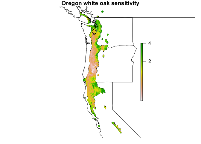
departureThe departure function provides a measure of a species’
potential exposure to climate change. It takes a future climate dataset
as an additional argument, and calculates the absolute differences
between historical and future values.
dep <- departure(x = climdat.hist, y = climdat.fut, s.dat = QUGA, field = "CODE")
dep
#> CLIMATIC DEPARTURE
#>
#> Departure factor:
#>   MDR   ISO    TS HMmax CMmin   PWM   PDM    PS   PWQ   PDQ
#>  0.05  0.10  0.22  0.53  0.44  0.23  0.12  0.38  0.23  0.16
#>
#> Overall departure: 0.909
The departure factor tells us the average amount of change that is
expected in each climate variable across the species’ range. Using the
exposure_map function, we can create a habitat map that
identifies where we expect the species to be most exposed to climate
change.
e.map <- exposure_map(dep)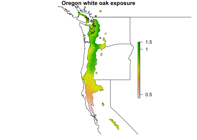
vulnerabilityThe vulnerability function provides a measure of a
species’ potential vulnerability to climate change, taking both
sensitivity and exposure into account. It takes a cnfa
object and a departure object as its arguments.
vuln <- vulnerability(cnfa = mod.cnfa, dep = dep)
vuln
#> CLIMATIC VULNERABILITY
#>
#> Vulnerability factor:
#>   MDR   ISO    TS HMmax CMmin   PWM   PDM    PS   PWQ   PDQ
#>  2.18  1.78  2.25  2.38  2.40  2.03  1.23  1.54  1.90  1.03
#>
#> Overall vulnerability: 1.368
Using the vulnerability_map function, we can create a
habitat map that identifies where we expect the species to be most
vulnerable to climate change.
v.map <- vulnerability_map(vuln)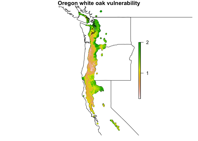
The raster package contains the clusterR
function, which enables parallelization methods for certain raster
operations. clusterR only works on functions that operate
on a cell-by-cell basis, however, which limits its usefulness. The
CENFA package contains a few functions that speed up some
basic raster functions considerably by parallelizing on a
layer-by-layer basis rather than a cell-by-cell basis.
parScaleThe parScale function is identical to
raster::scale, but has a parallelization option that will
scale each raster layer in parallel. The center and
scale arguments can be logical (TRUE or
FALSE) or numeric vectors.
clim.scaled <- parScale(x = climdat.hist, parallel = TRUE, n = 4)parCovThe parCov function returns the covariance matrix of a
Raster* object x, computing the covariance between each
layer of x. This is similar to
raster::layerStats(x, stat = 'cov'), but much faster when
parallelization is employed.
mat <- parCov(x = climdat.hist, parallel = TRUE, n = 4)Additionally, parCov can accept two Raster* objects as
arguments, similar to stats::cov(x, y). If two Raster*
objects are supplied, then the covariance is calculated between the
layers of x and the layers of y.
mat <- parCov(x = climdat.hist, y = climdat.fut, parallel = TRUE, n = 4)stretchPlotThe stretchPlot function provides a simple way to adjust
the contrast of plots of RasterLayers to emphasize difference in values.
It can perform histogram equalization and standard deviation
stretching.
sm <- sensitivity_map(mod.cnfa)
par(mfrow = c(1, 3), oma = c(1,1,1,1))
stretchPlot(sm, main = "linear")
stretchPlot(sm, type = "hist.equal", main = "Histogram equalization")
stretchPlot(sm, type = "sd", n = 2, main = "Standard deviation (n = 2)")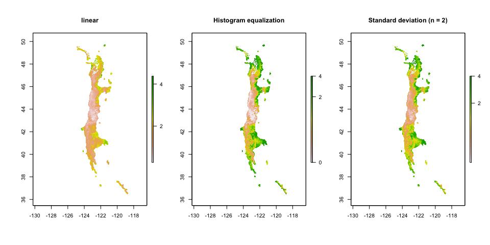
I welcome contributions and suggestions for improving this package. Please do not hesitate to submit any issues you may encounter.
Rinnan, D. Scott and Lawler, Joshua. Climate‐niche factor analysis: a spatial approach to quantifying species vulnerability to climate change. Ecography (2019). doi:10.1111/ecog.03937
Basille, Mathieu, et al. Assessing habitat selection using multivariate statistics: Some refinements of the ecological-niche factor analysis. Ecological Modelling 211.1 (2008): 233-240.
Hirzel, Alexandre H., et al. Ecological-niche factor analysis: how to compute habitat-suitability maps without absence data?. Ecology 83.7 (2002): 2027-2036.