![]()
![]()
activatr (pronounced like the word “activator”) is a
library for parsing GPX files into a standard format, and then
manipulating and visualizing those files.
You can install the released version of activatr from CRAN with:
install.packages("activatr")And the development version from GitHub with:
# install.packages("devtools")
devtools::install_github("dschafer/activatr")Basic parsing of a GPX file is simple: we use the
parse_gpx function and pass it the name of the GPX
file.
library(activatr)

# Get the running_example.gpx file included with this package.
filename <- system.file(
  "extdata",
  "running_example.gpx.gz",
  package = "activatr")

df <- parse_gpx(filename)
In its default configuration, parse_gpx will create a
row for every GPS point in the file, and pull out the latitude
(lat), longitude (lon), elevation
(ele, in meters), and time (time) into the
tibble:
| lat | lon | ele | time |
|---|---|---|---|
| 37.80405 | -122.4267 | 17.0 | 2018-11-03 14:24:45 |
| 37.80406 | -122.4267 | 16.8 | 2018-11-03 14:24:46 |
| 37.80408 | -122.4266 | 17.0 | 2018-11-03 14:24:48 |
| 37.80409 | -122.4266 | 17.0 | 2018-11-03 14:24:49 |
| 37.80409 | -122.4265 | 17.2 | 2018-11-03 14:24:50 |
We can also get a summary of the activity:
summary(df)| Distance | Date | Time | AvgPace | MaxPace | ElevGain | ElevLoss | AvgElev | Title |
|---|---|---|---|---|---|---|---|---|
| 9.407317 | 2018-11-03 14:24:45 | 4622s (~1.28 hours) | 491.319700444844s (~8.19 minutes) | 186.462178755299s (~3.11 minutes) | 188.364 | 253.4996 | -24.29198 | Sunrise 15K PR (sub-8:00) |
Once we have the data, it’s useful to visualize it. While basic visualizations work as expected with a data frame:
library(ggplot2)
qplot(lon, lat, data=df)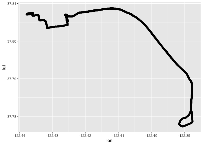
It’s more helpful to overlay this information on a correctly-sized
map. To aid in that, get_map_from_df gives us a
ggmap object (from the ggmap package), which
we can use to visualize our track.
Let’s see that on its own to start:
ggmap::ggmap(get_ggmap_from_df(df)) + theme_void()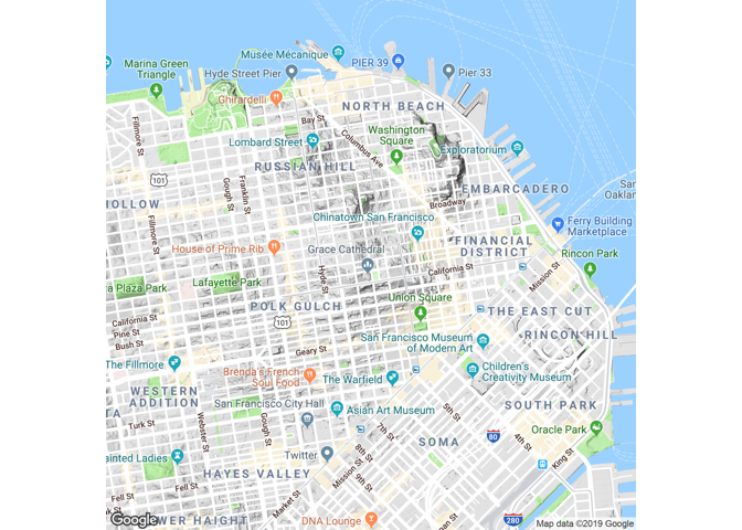
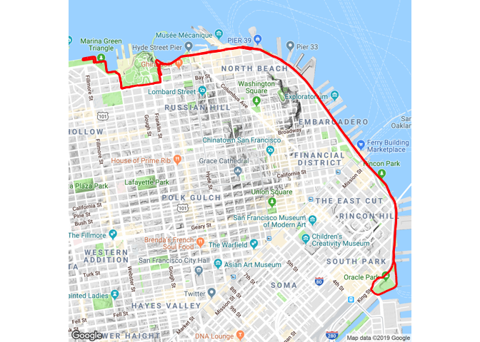
The axes show that we now have a ggmap at the right size to visualize the run. So putting it all together, we can make a nice basic graphic of the run:
ggmap::ggmap(get_ggmap_from_df(df)) +
  theme_void() +
  geom_path(aes(x = lon, y = lat), size = 1, data = df, color = "red")