Claudia Nunez-Penichet, Marlon E. Cobos, Jorge Soberon, Tomer Gueta, Narayani Barve, Vijay Barve, Adolfo G. Navarro-Siguenza, A. Townsend Peterson

This repository is for the project “Biological Survey Planning Considering Hutchinson’s Duality” developed during the program GSoC 2020 (see details at the end).
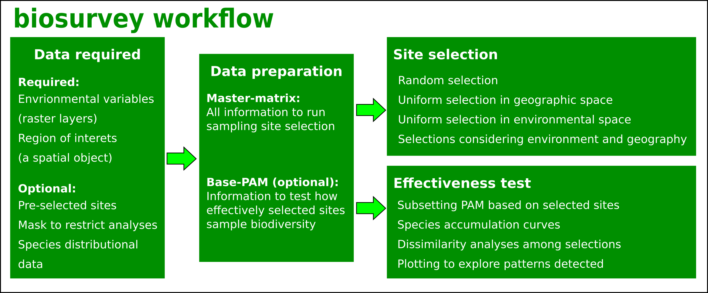
The biosurvey R package implements multiple tools to select sampling sites for biodiversity inventory, increasing effectiveness by considering the relationship of environmental and geographic conditions in a region. The functions are grouped in three main modules: 1) Data preparation; 2) Selection of sampling sites; and, 3) Tools for testing effectiveness (Fig. 1). Data are prepared in ways that avoid the need for more data in posterior analyses and allow users to focus on critical methodological decisions to select sampling sites. Various algorithms for selecting sampling sites are available, and options for considering pre-selected sites (known to be important for biodiversity monitoring) are included. Visualization is a critical component in this set of tools and most of the results obtained can be plotted to help users to understand their implications. The options for selecting sampling sites included here differ from other implementations in that they consider the environmental and geographic structure of a region to suggest sampling sites that could increase the effectiveness of efforts dedicated to inventor biodiversity.

Figure 1. Schematic view of the workflow to use biosurvey. Details on the workflow below.
Note: Internet connection is required to install the package.
To install the latest release of biosurvey use the following line of code:
# Installing from CRAN
install.packages("biosurvey")
The development version of biosurvey can be installed using the code below.
# Installing and loading packages
if(!require(remotes)){
  install.packages("remotes")
}

# To install the package use
remotes::install_github("claununez/biosurvey")

# To install the package and its vignettes use (if needed use: force = TRUE)
remotes::install_github("claununez/biosurvey", build_vignettes = TRUE)
If you have any problems during installation of the development
version from GitHub, restart R session, close other RStudio sessions you
may have open, and try again. If during the installation you are asked
to update packages, do so if you don’t need a specific version of one or
more of the packages to be installed. If any of the packages give an
error when updating, please install it alone using
install.packages(), then try installing
biosurvey again.
To load the package use:
# Load biosurvey
library(biosurvey)To check all functions in the package use:
help(biosurvey)If the package was installed with its vignettes you can see all options with:
vignette(package = "biosurvey")To check vignettes you can use:
vignette("biosurvey_preparing_data").- For a guide on
how to prepare data for analysis.vignette("biosurvey_selecting_sites").- For a guide on
how to select sampling sites.vignette("biosurvey_selection_with_preselected_sites").-
For a guide on how to select sampling sites when some sites have been
preselected.vignette("biosurvey_testing_module").- For a guide on
how to use the testing module.As shown in Fig. 1, to use biosurvey and select sites for biodiversity inventory you need:
stack from the
package raster.readOGR from the rgdal package.Additionally, other data can be used to make sampling site selection more effective. The functions that help to prepare the data for analysis also allow users to include:
If enough, good-quality data on species distributions are available, analyses of the effectiveness of sampling sites can be performed. The data used to prepare information to perform such analyses can be of different types:
To use biosurvey efficiently the first thing to do
is to prepare an object containing all information to be used in
following analyses. This can be done using the function
prepare_master_matrix(). After that, the function
make_blocks() can be used to partition the environmental
space of the region of interest. To explore how your data looks like,
the functions explore_data_EG() and
plot_blocks_EG() can be used.
After preparing data, distinct functions can be used to select sampling sites:
random_selection().- Random selection of sites to be
sampled in a survey.uniformG_selection().- Selection of sites with the goal
of maximizing uniformity of points in geographic space.uniformE_selection().- Selection of sites with the goal
of maximizing uniformity of points in environmental space.EG_selection().- Selection of sites with the goal of
maximizing uniformity of points in environment, but considering
geographic patterns of data.See also how your selected sites look like with the functions
plot_sites_EG(), plot_sites_E(), and
plot_sites_G().
After the selection of sampling sites, and, if enough high-quality data are available, functions from the testing module of this package can be used to explore which sets of sites selected could be better. Explore the following functions to prepare your data, and assess how well your selected sites perform in representing the exiting biodiversity:
prepare_base_PAM().- Prepares a presence-absence matrix
(PAM) from species distributional data; all sites (rows) will have a
value for presence or absence of species (columns).PAM_indices().- Calculates a set of biodiversity
indices using values contained in the presence-absence matrix.plot_PAM_geo().- Plot of PAM indices in geography.subset_PAM().- Subsets a base_PAM object according to
sites selected previously that are contained in a master_selection
object.selected_sites_SAC().- Creates species accumulation
curves for each set of selected sites contained in elements of
PAM_subset.plot_SAC().- Creates species accumulation curve plots
for selected sites.compare_SAC().- Creates comparative plots of two
species accumulation curves from information contained in lists obtained
with the function selected_sites_SAC().selected_sites_DI().- Computes dissimilarity indices
among sites selected and among sets of selected sites, based on the
communities of species represented in such units.plot_DI().- Creates matrix-like plots of
dissimilarities found among communities of species in distinct sites
selected or sets of sites selected.DI_dendrogram().- Plot dissimilarities withing and
among sets of selected sites as a dendrogram.Student: Claudia Nuñez-Penichet
GSoC Mentors: Narayani Barve, Vijay Barve, Tomer Gueta
Complete list of authors: Claudia Nunez-Penichet, Marlon E. Cobos, Jorge Soberon, Tomer Gueta, Narayani Barve, Vijay Barve, Adolfo G. Navarro-Siguenza, A. Townsend Peterson
Motivation:
Given the increasing intensity of threats to biodiversity in the world, one of the challenges in biodiversity conservation is to complete inventories of existing species at distinct scales. Species distributions depend on the relationships between accessible areas, environmental conditions, and biotic interactions. As planning a survey system only aims to register species in a region, biodiversity interaction can be overlooked in this case. However, the relationship between environmental conditions and the geographic configuration of an area is of crucial importance when trying to identify key sites for biodiversity surveys. Among the diverse packages in R for selecting survey sites, such considerations are not implemented and are limited to a random selection of sampling sites or analyses that allow detecting potential sampling sites based on the environmental similarity between sampled and unsampled areas. Given the need for more solutions, the biosurvey package aimed for considering the relationship between environmental and geographic conditions in a region when designing survey systems that allow sampling of most of its biodiversity.
At the moment we have completed the three main modules of the package. We have made modifications to the original list of products, which have helped us to improve the package functionality. The package is fully functional and available on CRAN.
All commits made can be seen at the complete list of commits.