
SHAP values (Lundberg and Lee, 2017) decompose model predictions into additive contributions of the features in a fair way. A model agnostic approach is called Kernel SHAP, introduced in Lundberg and Lee (2017), and investigated in detail in Covert and Lee (2021).
The “kernelshap” package implements a multidimensional refinement of the Kernel SHAP Algorithm described in Covert and Lee (2021). The package allows to calculate Kernel SHAP values in an exact way, by iterative sampling (as in Covert and Lee, 2021), or by a hybrid of the two. As soon as sampling is involved, the algorithm iterates until convergence, and standard errors are provided.
The default behaviour depends on the number of features \(p\):
The main function kernelshap() has three key
arguments:
object: Fitted model object.X: A (n x p) matrix,
data.frame, tibble or data.table
of rows to be explained. The columns should only represent model
features, not the response.bg_X: Background data used to integrate out “switched
off” features, often a subset of the training data (typically 50 to 500
rows). It should contain the same columns as X. In cases
with a natural “off” value (like MNIST digits), this can also be a
single row with all values set to the off value.Additional arguments of kernelshap() can be used to
control details of the algorithm, to activate parallel processing, or to
manually pass a prediction function.
Remarks
bg_w allows to weight background data according
to case weights.# From CRAN
install.packages("kernelshap")
# Or the newest version from GitHub:
# install.packages("devtools")
devtools::install_github("mayer79/kernelshap")The typical workflow to explain any model with Kernel SHAP:
object on some
training data, e.g., a linear regression, an additive model, a random
forest or a deep neural net. The only requirement is that predictions
are numeric.X to be explained. If the training dataset is small, simply
use the full training data for this purpose. X should only
contain feature columns.bg_X to calculate
marginal means. For this purpose, set aside 50 to 500 rows from the
training data. If the training data is small, use the full training
data.kernelshap(object, X, bg_X, ...) to calculate SHAP values.
Runtime is proportional to nrow(X), while memory
consumption scales linearly in nrow(bg_X).Let’s illustrate this on the diamonds data in the “ggplot2” package.
library(ggplot2)
library(kernelshap)
library(shapviz)

# Prepare data
diamonds <- transform(
  diamonds,
  log_price = log(price),
  log_carat = log(carat)
)

# 1) Fit model
fit_lm <- lm(log_price ~ log_carat + clarity + color + cut, data = diamonds)

# 2) Sample rows to be explained
set.seed(10)
xvars <- c("log_carat", "clarity", "color", "cut")
X <- diamonds[sample(nrow(diamonds), 1000), xvars]

# 3) Select background data
bg_X <- diamonds[sample(nrow(diamonds), 200), ]

# 4) Crunch SHAP values for all 1000 rows of X (~6 seconds)
system.time(
  shap_lm <- kernelshap(fit_lm, X, bg_X = bg_X)
)
shap_lm

# SHAP values of first 2 observations:
#           carat    clarity       color         cut
# [1,]  1.2692479  0.1081900 -0.07847065 0.004630899
# [2,] -0.4499226 -0.1111329  0.11832292 0.026503850

# 5) SHAP analysis
sv_lm <- shapviz(shap_lm)
sv_importance(sv_lm)
sv_dependence(sv_lm, "log_carat")
# ... more dependence plots
We can also explain a specific prediction instead of the full model:
single_row <- diamonds[5000, xvars]

fit_lm |>
  kernelshap(single_row, bg_X = bg_X) |>
  shapviz() |>
sv_waterfall()We can use the same X and bg_X to inspect
other models:
library(ranger)

# 1) Fit
fit_rf <- ranger(
  log_price ~ log_carat + clarity + color + cut,
  data = diamonds,
  num.trees = 20,
  seed = 20
)

# 4) Crunch
shap_rf <- kernelshap(fit_rf, X, bg_X = bg_X)
shap_rf

# SHAP values of first 2 observations:
#       log_carat     clarity      color         cut
# [1,]  1.1987785  0.09578879 -0.1397765 0.002761832
# [2,] -0.4969451 -0.12006207  0.1050928 0.029680717

# 5) Analyze
sv_rf <- shapviz(shap_rf)
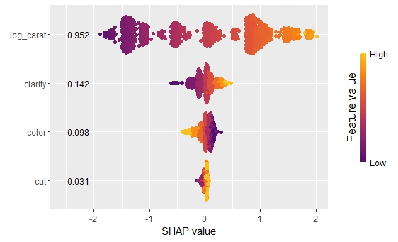
sv_importance(sv_rf, kind = "bee", show_numbers = TRUE)
sv_dependence(sv_rf, "log_carat", color_var = "auto")
# More dependence plots
Or a deep neural net (results not fully reproducible):
library(keras)

# 1) Fit
nn <- keras_model_sequential()
nn |>
  layer_dense(units = 30, activation = "relu", input_shape = 4) |>
  layer_dense(units = 15, activation = "relu") |>
  layer_dense(units = 1)

nn |>
  compile(optimizer = optimizer_adam(0.1), loss = "mse")

cb <- list(
  callback_early_stopping(patience = 20),
  callback_reduce_lr_on_plateau(patience = 5)
)

nn |>
  fit(
    x = data.matrix(diamonds[xvars]),
    y = diamonds$log_price,
    epochs = 100,
    batch_size = 400,
    validation_split = 0.2,
    callbacks = cb
  )

# 4) Crunch
pred_fun <- function(mod, X) predict(mod, data.matrix(X), batch_size = 10000)
shap_nn <- kernelshap(nn, X, bg_X = bg_X, pred_fun = pred_fun)

# 5) Analyze
sv_nn <- shapviz(shap_nn)
sv_importance(sv_nn, show_numbers = TRUE)
sv_dependence(sv_nn, "clarity", color_var = "auto")
# More dependence plotsAs long as you have set up a parallel processing backend, parallel
computing is supported via foreach. This will deactivate
the progress bar.
library(doFuture)

# Set up parallel backend
registerDoFuture()
plan(multisession, workers = 4)  # Windows
# plan(multicore, workers = 4)   # Linux, macOS, Solaris

# 4) Crunch with parallel computing (~3 seconds on second run)
system.time(
  s <- kernelshap(fit_lm, X, bg_X = bg_X, parallel = TRUE)
)On Windows, sometimes not all packages or global objects are passed
to the parallel sessions. In this case, the necessary instructions to
foreach can be specified through a named list via
parallel_args, see the following example:
library(mgcv)

# 1) Fit
fit_gam <- gam(log_price ~ s(log_carat) + clarity + color + cut, data = diamonds)

# 4) Crunch
system.time(
  shap_gam <- kernelshap(
    fit_gam,
    X,
    bg_X = bg_X,
    parallel = TRUE,
    parallel_args = list(.packages = "mgcv")
  )
)

shap_gam

# SHAP values of first 2 observations:
#       log_carat    clarity       color         cut
# [1,]  1.2714988  0.1115546 -0.08454955 0.003220451
# [2,] -0.5153642 -0.1080045  0.11967804 0.031341595

# 5) Analyze
# ...In above examples, since \(p\) was
small, exact Kernel SHAP values were calculated. Here, we want to show
how to use the different strategies (exact, hybrid, and pure sampling)
in a situation with ten features, see ?kernelshap for
details about those strategies. The results will be mostly identical.
Thus, you usually do not need to care about those options of
kernelshap().
With ten features, a degree 2 hybrid is used by default:
library(kernelshap)

set.seed(1)
X <- data.frame(matrix(rnorm(1000), ncol = 10))
y <- rnorm(10000L)
fit <- lm(y ~ ., data = cbind(y = y, X))

s <- kernelshap(fit, X[1L, ], bg_X = X)
summary(s)
s$S[1:5]
# Kernel SHAP values by the hybrid strategy of degree 2
#   - SHAP matrix of dim 1 x 10
#   - baseline: -0.005390948
#   - average number of iterations: 2
#   - rows not converged: 0
#   - proportion exact: 0.9487952
#   - m/iter: 20
#   - m_exact: 110
# 0.0101998581  0.0027579289 -0.0002294437  0.0005337086  0.0001179876
The algorithm converged in the minimal possible number of two
iterations and used \(110 + 2\cdot 20 =
150\) on-off vectors \(z\). For
each \(z\), predictions on a data set
with the same size as the background data are done. Three calls to
predict() were necessary (one for the exact part and one
per sampling iteration).
Since \(p\) is not very large in this case, we can also force the algorithm to use exact calculations:
s <- kernelshap(fit, X[1L, ], bg_X = X, exact = TRUE)
summary(s)
s$S[1:5]
# Exact Kernel SHAP values
#   - SHAP matrix of dim 1 x 10
#   - baseline: -0.005390948
#   - m_exact: 1022
# 0.0101998581  0.0027579289 -0.0002294437  0.0005337086  0.0001179876
The results are identical. While more on-off vectors \(z\) were required (1022), only a single
call to predict() was necessary.
Pure sampling (not recommended!) can be enforced by setting the hybrid degree to 0:
s <- kernelshap(fit, X[1L, ], bg_X = X, hybrid_degree = 0)
summary(s)
s$S[1:5]
# Kernel SHAP values by iterative sampling
#   - SHAP matrix of dim 1 x 10
#   - baseline: -0.005390948
#   - average number of iterations: 2
#   - rows not converged: 0
#   - proportion exact: 0
#   - m/iter: 80
#   - m_exact: 0
# 0.0101998581  0.0027579289 -0.0002294437  0.0005337086  0.0001179876
The results are again identical here and the algorithm converged in
two steps. In this case, two calls to predict() were
necessary and a total of 160 \(z\)
vectors were required.
Here, we provide some working examples for “tidymodels”, “caret”, and “mlr3”:
library(tidymodels)
library(kernelshap)

iris_recipe <- iris %>%
  recipe(Sepal.Length ~ .)

reg <- linear_reg() %>%
  set_engine("lm")

iris_wf <- workflow() %>%
  add_recipe(iris_recipe) %>%
  add_model(reg)

fit <- iris_wf %>%
  fit(iris)

ks <- kernelshap(fit, iris[, -1], bg_X = iris)
kslibrary(caret)
library(kernelshap)
library(shapviz)
fit <- train(
Sepal.Length ~ .,
data = iris,
method = "lm",
tuneGrid = data.frame(intercept = TRUE),
trControl = trainControl(method = "none")
)
s <- kernelshap(fit, iris[, -1], predict, bg_X = iris)
sv <- shapviz(s)
sv_waterfall(sv, 1)library(mlr3)
library(mlr3learners)
library(kernelshap)
library(shapviz)
mlr_tasks$get("iris")
tsk("iris")
task_iris <- TaskRegr$new(id = "iris", backend = iris, target = "Sepal.Length")
fit_lm <- lrn("regr.lm")
fit_lm$train(task_iris)
s <- kernelshap(fit_lm, iris[-1], bg_X = iris)
sv <- shapviz(s)
sv_dependence(sv, "Species")[1] Scott M. Lundberg and Su-In Lee. A Unified Approach to Interpreting Model Predictions. Advances in Neural Information Processing Systems 30, 2017.
[2] Ian Covert and Su-In Lee. Improving KernelSHAP: Practical Shapley Value Estimation Using Linear Regression. Proceedings of The 24th International Conference on Artificial Intelligence and Statistics, PMLR 130:3457-3465, 2021.