
![]()
![]()

Empirical likelihood enables a nonparametric, likelihood-driven style of inference without relying on assumptions frequently made in parametric models. Empirical likelihood-based tests are asymptotically pivotal and thus avoid explicit studentization. For this reason it is challenging to incorporate empirical likelihood methods directly into other packages that perform inferences for parametric models. The R package melt aims to bridge the gap and provide a unified framework for data analysis with empirical likelihood methods. A collection of functions are available to perform multiple empirical likelihood tests and construct confidence intervals for linear and generalized linear models in R. The package offers an easy-to-use interface and flexibility in specifying hypotheses and calibration methods, extending the framework to simultaneous inferences. The core computational routines are implemented with the Eigen C++ library and RcppEigen interface, with OpenMP for parallel computation. Details of the testing procedures are given in Kim, MacEachern, and Peruggia (2021). This work was supported by the U.S. National Science Foundation under Grants No. SES-1921523 and DMS-2015552.
You can install the latest stable release from CRAN.
install.packages("melt")You can install the latest development version from GitHub or R-universe.
# install.packages("devtools")
devtools::install_github("ropensci/melt")install.packages("melt", repos = "https://ropensci.r-universe.dev")melt provides an intuitive API for performing the most common data analysis tasks:
el_lm() fits a linear model with empirical
likelihood.el_glm() fits a generalized linear model with empirical
likelihood.confint() computes confidence intervals for model
parameters.confreg() computes confidence region for model
parameters.elt() tests a linear hypothesis.elmt() performs multiple testing simultaneously.library(melt)
set.seed(971112)
## Test for the mean
data("precip")
el_mean(precip, par = 30)
#>
#> Empirical Likelihood
#>
#> Model: mean
#>
#> Maximum EL estimates:
#> [1] 34.89
#>
#> Chisq: 8.285, df: 1, Pr(>Chisq): 0.003998
#>
#> EL evaluation: converged
## Linear model
data("mtcars")
fit_lm <- el_lm(mpg ~ disp + hp + wt + qsec, data = mtcars)
summary(fit_lm)
#>
#> Call:
#> el_lm(formula = mpg ~ disp + hp + wt + qsec, data = mtcars)
#>
#> Coefficients:
#> Estimate Chisq Pr(>Chisq)
#> (Intercept) 27.329638 443.208 < 2e-16 ***
#> disp 0.002666 0.365 0.54575
#> hp -0.018666 10.730 0.00105 **
#> wt -4.609123 439.232 < 2e-16 ***
#> qsec 0.544160 440.583 < 2e-16 ***
#> ---
#> Signif. codes: 0 '***' 0.001 '**' 0.01 '*' 0.05 '.' 0.1 ' ' 1
#> Chisq: 433.4, df: 4, Pr(>Chisq): < 2.2e-16
#>
#> Constrained EL: converged
cr <- confreg(fit_lm, parm = c("disp", "hp"), npoints = 200)
plot(cr)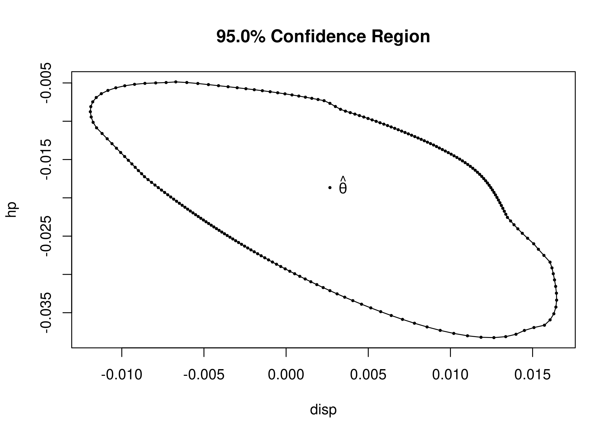
data("clothianidin")
fit2_lm <- el_lm(clo ~ -1 + trt, data = clothianidin)
summary(fit2_lm)
#>
#> Call:
#> el_lm(formula = clo ~ -1 + trt, data = clothianidin)
#>
#> Coefficients:
#>              Estimate   Chisq Pr(>Chisq)
#> trtNaked       -4.479 411.072    < 2e-16 ***
#> trtFungicide   -3.427  59.486   1.23e-14 ***
#> trtLow         -2.800  62.955   2.11e-15 ***
#> trtHigh        -1.307   4.653      0.031 *
#> ---
#> Signif. codes:  0 '***' 0.001 '**' 0.01 '*' 0.05 '.' 0.1 ' ' 1
#> Chisq: 894.4, df: 4, Pr(>Chisq): < 2.2e-16
#>
#> EL evaluation: not converged
confint(fit2_lm)
#>                  lower      upper
#> trtNaked     -5.002118 -3.9198229
#> trtFungicide -4.109816 -2.6069870
#> trtLow       -3.681837 -1.9031795
#> trtHigh      -2.499165 -0.1157222


## Generalized linear model
data("thiamethoxam")
fit_glm <- el_glm(visit ~ log(mass) + fruit + foliage + var + trt,
  family = quasipoisson(link = "log"), data = thiamethoxam,
  control = el_control(maxit = 100, tol = 1e-08, nthreads = 4)
)
summary(fit_glm)
#>
#> Call:
#> el_glm(formula = visit ~ log(mass) + fruit + foliage + var +
#>     trt, family = quasipoisson(link = "log"), data = thiamethoxam,
#>     control = el_control(maxit = 100, tol = 1e-08, nthreads = 4))
#>
#> Coefficients:
#>              Estimate   Chisq Pr(>Chisq)
#> (Intercept)   0.74032 189.226    < 2e-16 ***
#> log(mass)     0.16938 401.439    < 2e-16 ***
#> fruit         0.04043  10.044    0.00153 **
#> foliage     -10.84203   5.805    0.01598 *
#> varGZ        -0.60770  37.549   8.92e-10 ***
#> trtSpray      0.06370   0.505    0.47730
#> trtFurrow    -0.04124   0.084    0.77170
#> trtSeed       0.14281   1.276    0.25857
#> ---
#> Signif. codes:  0 '***' 0.001 '**' 0.01 '*' 0.05 '.' 0.1 ' ' 1
#>
#> Dispersion estimate for quasipoisson family: 1.316692
#>
#> Chisq: 117.2, df: 7, Pr(>Chisq): < 2.2e-16
#>
#> Constrained EL: converged


## Test of no treatment effect
contrast <- c(
  "trtNaked - trtFungicide", "trtFungicide - trtLow", "trtLow - trtHigh"
)
elt(fit2_lm, lhs = contrast)
#>
#>  Empirical Likelihood Test
#>
#> Hypothesis:
#> trtNaked - trtFungicide = 0
#> trtFungicide - trtLow = 0
#> trtLow - trtHigh = 0
#>
#> Significance level: 0.05, Calibration: Chi-square
#>
#> Statistic: 26.6, Critical value: 7.815
#>
#> p-value: 7.148e-06


## Multiple testing
contrast2 <- rbind(
  c(0, 0, 0, 0, 0, 1, 0, 0),
  c(0, 0, 0, 0, 0, 0, 1, 0),
  c(0, 0, 0, 0, 0, 0, 0, 1)
)
elmt(fit_glm, lhs = contrast2)
#>
#>  Empirical Likelihood Multiple Tests
#>
#> Overall significance level: 0.05
#>
#> Calibration: Multivariate chi-square
#>
#> Hypotheses:
#>               Estimate Chisq Df p.adj
#> trtSpray = 0   0.06370 0.471  1 0.849
#> trtFurrow = 0 -0.04124 0.078  1 0.987
#> trtSeed = 0    0.14281 1.276  1 0.558
#>
#> Common critical value: 5.612
Please note that this package is released with a Contributor Code of Conduct. By contributing to this project, you agree to abide by its terms.