
{migraph} works with and extends existing network
analysis packages for analysing multimodal networks. It provides a
common, standard syntax for working with and analysing both one-mode and
two-mode networks.
The package is intended as a software companion to the book:
David Knoke, Mario Diani, James Hollway, and Dimitris Christopoulos (2021) Multimodal Political Networks. Cambridge University Press: Cambridge.
Most datasets used in the book are included in this package, and the package implements most methods discussed in the book. Since many of theses datasets and routines are discussed and analysed more there, if you like the package please check out the book, and vice versa.
{migraph} can help with many network analytic tasks,
including Making and Manipulating network data, Marking and Measuring
nodes, ties, and networks, calculating Motifs and identifying
Memberships, as well as Modelling and Mapping.
{migraph} includes a number of prominent network
datasets, especially multimodal and multiplex examples for demonstrating
more advanced methods.
mpn_bristol, mpn_cow_igo,
mpn_cow_trade, mpn_DE_1990,
mpn_DE_2008, mpn_DemSxP,
mpn_elite_mex, mpn_elite_usa_advice,
mpn_elite_usa_money, mpn_IT_1990,
mpn_IT_2008, mpn_OverSxP,
mpn_RepSxP, mpn_ryanair,
mpn_UK_1990, mpn_UK_2008ison_adolescents, ison_algebra,
ison_bb, ison_bm, ison_brandes,
ison_brandes2, ison_karateka,
ison_lotr, ison_marvel_relationships,
ison_marvel_teams, ison_mb,
ison_mm, ison_networkers,
ison_southern_womenIf that’s not enough, {migraph} offers a number of
options for importing network data found in other repositories.
{migraph} can import and export to Excel edgelists and
nodelists, UCINET, Pajek, and DynetML files,
e.g.:
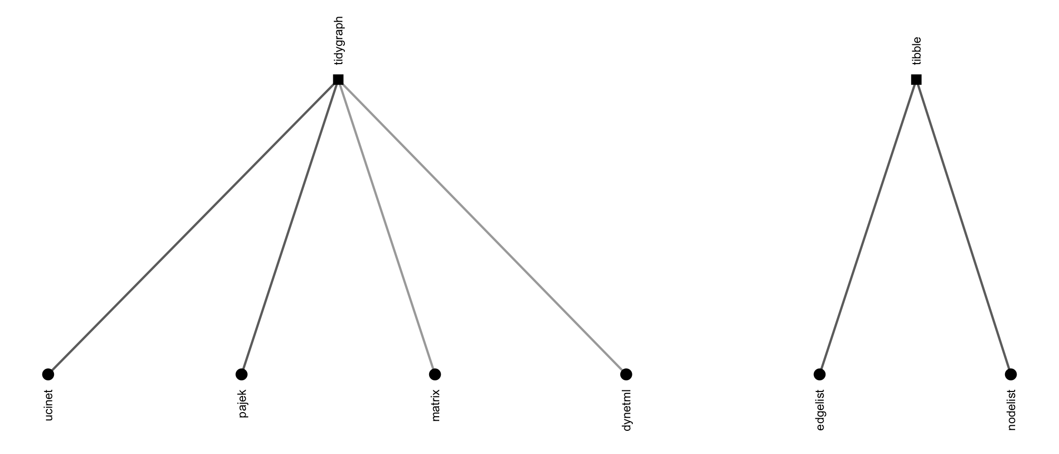
read_dynetml(), read_edgelist(),
read_matrix(), read_nodelist(),
read_pajek(), read_ucinet()write_edgelist(), write_nodelist(),
write_pajek(), write_ucinet(){migraph} includes algorithms for making networks with
particular properties. The create_* group of functions
create networks with a particular structure, e.g.:
create_complete(), create_components(),
create_core(), create_empty(),
create_lattice(), create_ring(),
create_star(), create_tree()The generate_* group of functions generate networks from
particular generative mechanisms, e.g.:
generate_permutation(), generate_random(),
generate_scalefree(),
generate_smallworld()Note that all these functions work to create two-mode networks as well as one-mode versions.
In addition to functions that help add elements to or extract
elements from a network, {migraph} also includes functions
for coercing and changing network data.
Once network data is in R, {migraph}’s
as_*() functions can be used to translate objects from one
of the above classes into any other, and include:
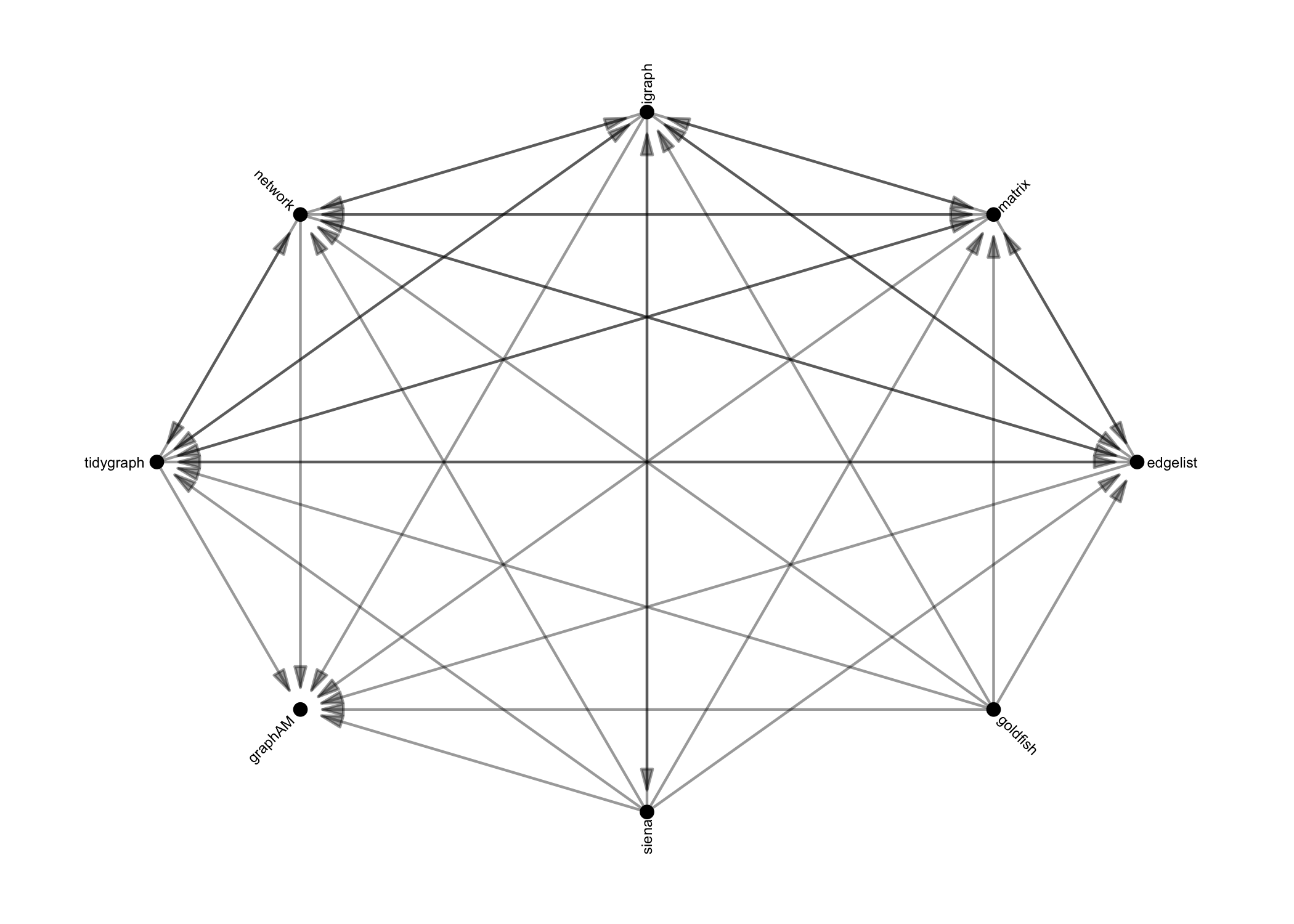
These functions are designed to be as intuitive and lossless as possible, outperforming many other class-coercion packages.
We use these functions internally in every {migraph}
function to (1) allow them to be run on any compatible network format
and (2) use the most efficient algorithm available. This makes
{migraph} compatible with your existing workflow, whether
you use base R matrices or edgelists as data frames, {igraph}, {network}, or {tidygraph},
and extensible by developments in those other packages too.
{migraph}’s to_*() functions can be used on
any class object to reformat, transform, or split networks into networks
with other properties, e.g.:
to_anti(), to_blocks(),
to_components(), to_edges(),
to_egos(), to_giant(),
to_main_component(), to_matching(),
to_mode1(), to_mode2(),
to_multilevel(), to_named(),
to_onemode(), to_redirected(),
to_simplex(), to_subgraph(),
to_subgraphs(), to_ties(),
to_twomode(), to_undirected(),
to_uniplex(), to_unnamed(),
to_unsigned(), to_unweighted()Reformatting means changing the format of the network, e.g. from
directed to undirected via to_undirected(). Transforming
means changing the dimensions of the network, e.g. from a two-mode
network to a one-mode projection via to_mode1(). Splitting
means separating a network, e.g. from a whole network to the various ego
networks via to_egos(). Those functions that split a
network into a list of networks are distinguishable as those
to_*() functions that are named in the plural.
{migraph} offers a range of measures and models with
sensible defaults. Many wrap existing functions in common packages for
use with one-mode networks, but extend these to treat and/or normalise
for two-mode (and sometimes three-mode) networks correctly. Functions
are given intuitive and succinct names that avoid conflicts with
existing function names wherever possible.
{migraph}’s *is_*() functions offer fast
logical tests of various properties. Whereas is_*() returns
a single logical value for the network, node_is_*() returns
a logical vector the length of the number of nodes in the network, and
tie_is_*() returns a logical vector the length of the
number of ties in the network.
is_acyclic(), is_aperiodic(),
is_bipartite(), is_complex(),
is_connected(), is_directed(),
is_edgelist(), is_eulerian(),
is_graph(), is_labelled(),
is_migraph(), is_multiplex(),
is_perfect_matching(), is_signed(),
is_twomode(), is_uniplex(),
is_weighted()node_is_core(), node_is_cutpoint(),
node_is_isolate(), node_is_max(),
node_is_min(), node_is_random()tie_is_bridge(), tie_is_loop(),
tie_is_max(), tie_is_min(),
tie_is_multiple(), tie_is_reciprocated()The *is_max() and *is_min() functions are
used to identify the maximum or minimum, respectively, node or tie
according to some measure (see below).
{migraph} offers a large and growing smorgasbord of
measures that can be used at the node, tie, and network level. Each
recognises whether the network is directed or undirected, weighted or
unweighted, one-mode or two-mode. All return normalized values wherever
possible, though this can be overrided. Here are some examples:
node_degree(),
node_closeness(), node_betweenness(), and
node_eigenvector()network_degree(),
network_closeness(), network_betweenness(),
and network_eigenvector()network_density(),
network_reciprocity(), network_transitivity(),
network_equivalency(), and
network_congruency()network_components(),
network_cohesion(), network_adhesion(),
network_diameter(), network_length()network_diversity(),
network_homophily(), network_assortativity(),
node_diversity(), node_homophily(),
node_assortativity(), node_richness()node_redundancy(),
node_effsize(), node_efficiency(),
node_constraint(), node_hierarchy()network_core(),
network_factions(), network_modularity(),
network_smallworld(), network_balance()Please explore the list of functions to find out more.
The package also include functions for returning various censuses at the network or node level, e.g.:
network_brokerage_census(),
network_dyad_census(), network_mixed_census(),
network_triad_census()node_brokerage_census(),
node_path_census(), node_quad_census(),
node_tie_census(), node_triad_census()These can be analysed alone, or used as a profile for establishing
equivalence. {migraph} offers both HCA and CONCOR
algorithms, as well as elbow, silhouette, and strict methods for
k-cluster selection.
node_automorphic_equivalence(),
node_equivalence(),
node_regular_equivalence(),
node_structural_equivalence(){migraph} also includes functions for establishing
membership on other bases, such as typical community detection
algorithms, as well as component and core-periphery partitioning
algorithms.
All measures can be tested against conditional uniform graph (CUG) or quadratic assignment procedure (QAP) distributions using:
test_permutation(), test_random()Hypotheses can also be tested within multivariate models via multiple (linear or logistic) regression QAP:
network_reg(){migraph} is the only package that offers these testing
frameworks for two-mode networks as well as one-mode networks.
Lastly, {migraph} also includes functions for simulating
diffusion or learning processes over a given network:
play_diffusion(), play_diffusions(),
play_learning()The diffusion models include not only SI and threshold models, but also SIS, SIR, SIRS, SIER, and SIERS.
Plot methods for all outputs assist with interpretation and communication.
Besides intuitive plot() methods for most of the above
outputs, {migraph} also includes autographr()
for one-line plotting graphs with sensible defaults based on their
properties. {migraph} uses the excellent
{ggraph} package (and thus {ggplot2}) as a
plotting engine. This also makes extending and theming default output
easy, and {patchwork} is used to help arrange individual
plots together.
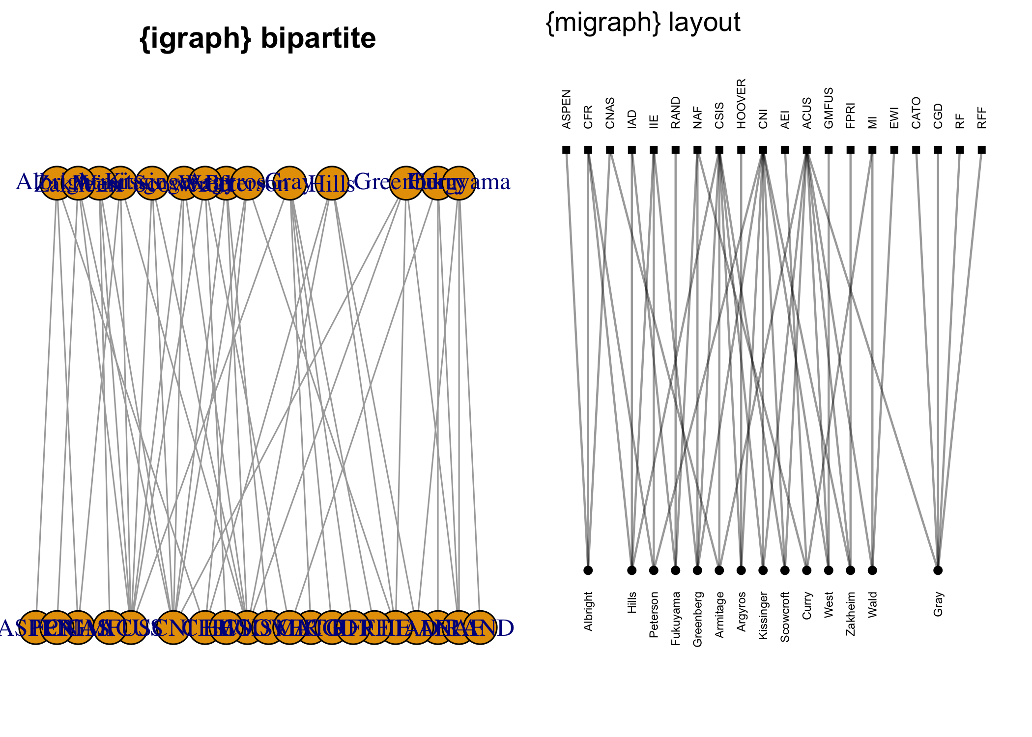
In addition, {migraph} offers some additional layout
algorithms for snapping layouts to a grid or visualising partitions
horizontally, vertically, or concentrically. The following figures
illustrate the difference in results over {igraph}:
The easiest way to install the latest stable version of
{migraph} is via CRAN. Simply open the R console and
enter:
install.packages('migraph')
You can then begin to use {migraph} by loading the
package:
library(migraph)
This will load any required packages and make the data contained within the package available. The version from CRAN also has all the vignettes built and included. You can check them out with:
vignettes(package = "migraph")
For the latest development version, for slightly earlier access to new features or for testing, you may wish to download and install the binaries from Github or install from source locally.
The latest binary releases for all major OSes – Windows, Mac, and Linux – can be found here. Download the appropriate binary for your operating system, and install using an adapted version of the following commands:
install.packages("~/Downloads/migraph_winOS.zip", repos = NULL)install.packages("~/Downloads/migraph_macOS.tgz", repos = NULL)install.packages("~/Downloads/migraph_linuxOS.tar.gz", repos = NULL)To install from source the latest main version of
{migraph} from Github, please install the
{remotes} or {devtools} package from CRAN and
then:
remotes::install_github("snlab-ch/migraph", build_vignettes = TRUE)remotes::install_github("snlab-ch/migraph@develop", build_vignettes = TRUE)This package has recently moved away from the use of vignettes, in
favour of smaller and more interactive {learnr} tutorials.
Since version 0.12.3, many of the previous vignettes are instead
available as tutorials, more will be converted soon, and those that have
been converted will continue to be updated and enriched.
To access the tutorials, you will need to have the additional package
{learnr} installed:
install.packages("learnr"). Then we would first suggest
that you check to see which vignettes are currently available:
learnr::available_tutorials("migraph")
#> Available tutorials:
#> * migraph
#>   - tutorial2 : "Visualisation"
#>   - tutorial3 : "Centrality"
#>   - tutorial4 : "Community"
#>   - tutorial5 : "Equivalence"
#>   - tutorial6 : "Topology"
#>   - tutorial7 : "Diffusion"
#>   - tutorial8 : "Regression"
You can then choose to begin a tutorial using the following command:
e.g. learnr::run_tutorial("tutorial2", "migraph"). For more
details on the {learnr} package, see here.
It draws together, updates, and builds upon many functions currently
available in other excellent R packages such as {bipartite},
{multinet},
and {tnet}, and
implements many additional features currently only available outside the
R ecosystem in packages such as UCINET.
Subsequent work on this package has been funded by the Swiss National Science Foundation (SNSF) Grant Number 188976: “Power and Networks and the Rate of Change in Institutional Complexes” (PANARCHIC).