An R package for ordinal pattern analysis.
opa can be installed from CRAN with:
install.packages("opa")You can install the development version of opa from GitHub with:
# install.packages("remotes")
remotes::install_github("timbeechey/opa")To cite opa in your work you can use the output of:
citation(package = "opa")opa is an implementation of methods described in
publications including Thorngate
(1987) and Grice
et al. (2015). Thorngate (1987) attributes the original idea to:
Parsons, D. (1975). The directory of tunes and musical themes. S. Brown.
Ordinal pattern analysis is similar to Kendall’s Tau. Whereas Kendall’s tau is a measure of similarity between two data sets in terms of rank ordering, ordinal pattern analysis is intended to quantify the match between a hypothesis and patterns of individual-level data across conditions or measurement instances.
Ordinal pattern analysis works by comparing the relative ordering of pairs of observations and computing whether those pairwise relations are matched by a hypothesis. Each pairwise ordered relation is classified as an increases, a decrease, or as no change. These classifications are encoded as 1, -1 and 0, respectively. For example, a hypothesis of a monotonic increase in a response variable across four experimental conditions can be specified as:
h <- c(1, 2, 3, 4)Note that the absolute values are not important, only their relative
ordering. The hypothesis h encodes six pairwise relations,
all increases: 1 1 1 1 1 1.
A row of individual data representing measurements across four conditions, such as:
dat <- c(65.3, 68.8, 67.0, 73.1)encodes six ordered pairwise relations 1 1 1 -1 1 1. The
percentage of orderings which are correctly classified by the hypothesis
(PCC) is the main quantity of interest in ordinal pattern
analysis. Comparing h and dat, the PCC is
5/6 = 0.833 or 83.3%. A hypothesis which generates a
greater PCC is preferred over a hypothesis which generates a lower PCC
for given data.
It is also possible to calculate a chance-value for a PCC which is equal to the chance that a PCC at least as great as the PCC of the observed data could occur as a result of a random re-ordering of the data. Chance values can be computed using either a permutation test or a randomization test.
opalibrary(opa)A hypothesized relative ordering of a response variable across conditions is specified with a numeric vector:
h <- c(1, 2, 4, 3)The hypothesis can be plotted with the plot_hypothesis()
function:
plot_hypothesis(h)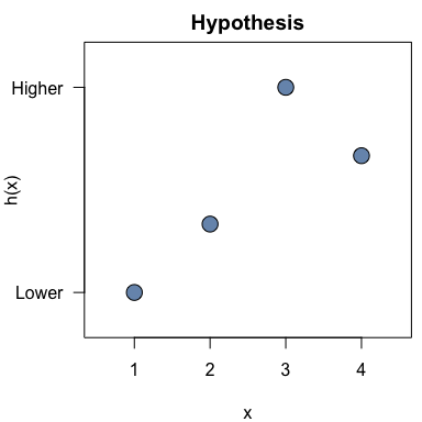
Data should be in wide format with one column per measurement condition and one row per individual:
set.seed(123)

dat <- data.frame(t1 = rnorm(20, mean = 12, sd = 2),
                  t2 = rnorm(20, mean = 15, sd = 2),
                  t3 = rnorm(20, mean = 20, sd = 2),
                  t4 = rnorm(20, mean = 17, sd = 2))

round(dat, 2)
#>       t1    t2    t3    t4
#> 1  10.88 12.86 18.61 17.76
#> 2  11.54 14.56 19.58 16.00
#> 3  15.12 12.95 17.47 16.33
#> 4  12.14 13.54 24.34 14.96
#> 5  12.26 13.75 22.42 14.86
#> 6  15.43 11.63 17.75 17.61
#> 7  12.92 16.68 19.19 17.90
#> 8   9.47 15.31 19.07 17.11
#> 9  10.63 12.72 21.56 18.84
#> 10 11.11 17.51 19.83 21.10
#> 11 14.45 15.85 20.51 16.02
#> 12 12.72 14.41 19.94 12.38
#> 13 12.80 16.79 19.91 19.01
#> 14 12.22 16.76 22.74 15.58
#> 15 10.89 16.64 19.55 15.62
#> 16 15.57 16.38 23.03 19.05
#> 17 13.00 16.11 16.90 16.43
#> 18  8.07 14.88 21.17 14.56
#> 19 13.40 14.39 20.25 17.36
#> 20 11.05 14.24 20.43 16.72
An ordinal pattern analysis model to consider how the hypothesis
h matches each individual pattern of results in
dat can be fitted using:
opamod <- opa(dat, h)Specifying cval_method = "exact" computes chance values
using a permutation test which considers every possible ordering of the
data to determine the exact chance of a PCC at least as high as the PCC
of the observed data. Specifying instead
cval_method = "stochastic" computes chance values based on
PCCs computed from a set of random orderings of the data. The number of
random orderings to consider can be specified with the
nreps argument which defaults to 1000L.
A summary of the model output can be viewed using:
summary(opamod)
#> Ordinal Pattern Analysis of 4 observations for 20 individuals in 1 group
#>
#> Between subjects results:
#>          PCC cval
#> pooled 93.33    0
#>
#> Within subjects results:
#>       PCC cval
#> 1  100.00 0.04
#> 2  100.00 0.03
#> 3   83.33 0.17
#> 4  100.00 0.05
#> 5  100.00 0.05
#> 6   83.33 0.17
#> 7  100.00 0.04
#> 8  100.00 0.04
#> 9  100.00 0.04
#> 10  83.33 0.19
#> 11 100.00 0.06
#> 12  66.67 0.37
#> 13 100.00 0.04
#> 14  83.33 0.18
#> 15  83.33 0.17
#> 16 100.00 0.04
#> 17 100.00 0.04
#> 18  83.33 0.17
#> 19 100.00 0.04
#> 20 100.00 0.05
#>
#> PCCs were calculated for pairwise ordinal relationships using a difference threshold of 0.
#> Chance-values were calculated using the stochastic method.
Individual-level model output can be plotted using:
plot(opamod)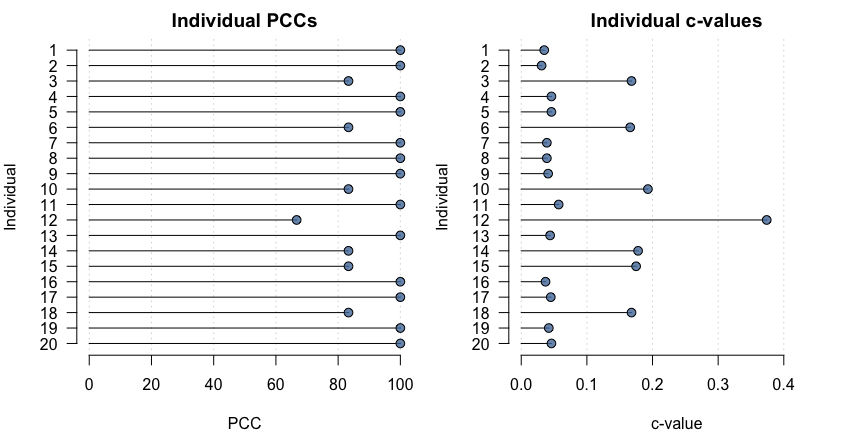
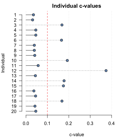
To aid in visual interpretation, individual PCCs and c-values can also be plotted relative to user-specified thresholds:
pcc_plot(opamod, threshold = 90)
cval_plot(opamod, threshold = 0.1)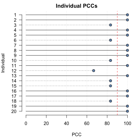
Pairwise comparisons of measurement conditions can be calculated by
applying the compare_conditions() function to an
opafit object produced by a call to opa():
condition_comparisons <- compare_conditions(opamod)

condition_comparisons$pccs
#>     1   2  3 4
#> 1   -   -  - -
#> 2  90   -  - -
#> 3 100 100  - -
#> 4  95  80 95 -
condition_comparisons$cvals
#>   1     2 3 4
#> 1 -     - - -
#> 2 0     - - -
#> 3 0     0 - -
#> 4 0 0.002 0 -If the data consist of multiple groups a categorical grouping
variable can be passed with the group keyword to produce
results for each group within the data, in addition to individual
results.
dat$group <- rep(c("A", "B", "C", "D"), 5)
dat$group <- factor(dat$group, levels = c("A", "B", "C", "D"))

opamod2 <- opa(dat[, 1:4], h, group = dat$group)
The summary output displays results organised by group.
summary(opamod2, digits = 3)
#> Ordinal Pattern Analysis of 4 observations for 20 individuals in 4 groups
#>
#> Between subjects results:
#>       PCC  cval
#> A 100.000 0.000
#> B  86.667 0.001
#> C  93.333 0.000
#> D  93.333 0.000
#>
#> Within subjects results:
#>   Individual     PCC  cval
#> A          1 100.000 0.042
#> A          5 100.000 0.044
#> A          9 100.000 0.041
#> A         13 100.000 0.041
#> A         17 100.000 0.044
#> B          2 100.000 0.049
#> B          6  83.333 0.177
#> B         10  83.333 0.160
#> B         14  83.333 0.166
#> B         18  83.333 0.154
#> C          3  83.333 0.184
#> C          7 100.000 0.047
#> C         11 100.000 0.035
#> C         15  83.333 0.149
#> C         19 100.000 0.037
#> D          4 100.000 0.040
#> D          8 100.000 0.043
#> D         12  66.667 0.374
#> D         16 100.000 0.034
#> D         20 100.000 0.039
#>
#> PCCs were calculated for pairwise ordinal relationships using a difference threshold of 0.
#> Chance-values were calculated using the stochastic method.
Similarly, plotting the output shows individual PCCs and c-values by group.
plot(opamod2)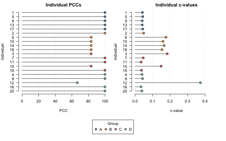
Development of opa was supported by a Medical Research
Foundation Fellowship (MRF-049-0004-F-BEEC-C0899).