The goal of pedbuildr is to reconstruct small/medium-sized pedigrees from genotype data.
The development version of pedbuildr is available from GitHub:
remotes::install_github("magnusdv/pedbuildr")Load the package into R as follows:
library(pedbuildr)
#> Loading required package: pedtoolsTo get started, we demonstrate how to reconstruct the pedigree
connecting three individuals from their genotypes at 100 SNP markers.
The (simulated) genotypes are contained in the dataset
trioData built-in to pedbuildr. Here are
the first few columns:
trioData[, 1:10]
#>   id fid mid sex <1> <2> <3> <4> <5> <6>
#> 1  1   0   0   1 1/2 1/2 1/1 1/2 1/2 1/2
#> 2  2   0   0   1 1/1 1/2 1/2 2/2 1/2 2/2
#> 3  3   0   0   1 1/1 1/2 1/2 2/2 1/1 1/2
The first thing to do is to convert the data into pedigree object,
using the as.ped() function from
pedtools.
x = as.ped(trioData, locusAttributes = "snp-12")
summary(x)
#> List of 3 singletons.
#> Labels: 1 (male), 2 (male), 3 (male).
#> 100 attached markers.
The locusAttributes argument tells R that all the
markers are diallelic with alleles 1 and 2. By default, the alleles have
equal frequencies.
To reconstruct the pedigree, simply run
reconstruct():
res = reconstruct(x)
#> Pedigree parameters:
#>   ID labels: 1, 2, 3
#>   Sex: 1, 1, 1
#>   Extra: parents
#>   Age info: -
#>   Known PO: -
#>   Known non-PO: -
#>   No children: -
#>   Connected only: TRUE
#>   Symmetry filter: TRUE
#>   Linear inbreeding: TRUE
#>
#> Building pedigree list:
#>   Undirected adjacency matrices: 8
#>   Directed adjacency matrices: 16
#>   After adding parents: 114
#>   Connected solutions: 95
#>
#> Computing the likelihood of 95 pedigrees.
#> Sorting by descending likelihood.
#> Total time used:  6.04 secs
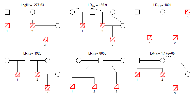
The most likely pedigrees are plotted as follows.
plot(res, top = 6)
A priori there are infinitely many possible pedigrees
connecting a set of individuals. (For example, two individuals may be
k’th cousins for any k = 1,2,… .) In order to obtain a
manageable search space, reconstruct() offers a range of
restriction parameters:
extra: The number of extra individuals allowed to
connect the original individuals. (See further explanations below.)age: A character vector describing age inequalities.
For example, age = c("A > B,C", "B > D") excludes B
and C as ancestors of A, and D as an ancestor of B (but no assumption is
made for C vs. D).inferPO: If TRUE, an initial stage of pairwise IBD
estimation is done, in order to infer certain parent-child pairs, as
well as certain non-parent-child pairs.knownPO: Known parent–offspring pairs.notPO: Pairs known not to be parent–offspring.allKnown: If TRUE, then knownPO is the
complete list of parent–offspring pairs.noChildren: Individuals known to have no children.linearInb: The allowed level of inbreeding between
linear descendants. For example, linearInb = 1 allows
mating between parent–child, but not grandparent–grandchild. Set to
FALSE to disallow all inbreeding of this type.connected: If TRUE (default), only connected pedigrees
are considered.sexSymmetry: If TRUE (default) pedigrees are considered
equal if they differ only in the sexes of the added parents, e.g.,
paternal versus maternal half-siblings.Let us re-run the reconstruction of trioData adding a
few of these restrictions. We allow 3 extra individuals and indicate
that individual 1 is older than the others. Furthermore, we ask the
program to infer parent-child relationships automatically, and disallow
linear inbreeding.
res2 = reconstruct(x, extra = 3, age = "1 > 2,3", inferPO = TRUE, linearInb = FALSE)
#> Pairwise estimation:
#>   PO: 2-3
#>   non-PO: 1-3
#>
#> Pedigree parameters:
#>   ID labels: 1, 2, 3
#>   Sex: 1, 1, 1
#>   Extra: 3
#>   Age info: 1>2, 1>3
#>   Known PO: 2-3
#>   Known non-PO: 1-3
#>   No children: -
#>   Connected only: TRUE
#>   Symmetry filter: TRUE
#>   Linear inbreeding: FALSE
#>
#> Building pedigree list:
#>   First 2: 2 candidates (0 secs)
#>   All 3 + 0 extra: 1 solutions | 3 candidates (0 secs)
#>   All 3 + 1 extra: 9 solutions | 30 candidates | 21 duplicates removed (0.0156 secs)
#>   All 3 + 2 extra: 35 solutions | 266 candidates | 501 duplicates removed (0.217 secs)
#>   All 3 + 3 extra: 183 solutions | 183 candidates | 459 duplicates removed (0.932 secs)
#> Total solutions: 228
#> Converting to ped
#> Total time: 0.991 secs
#> Computing the likelihood of 228 pedigrees.
#> Sorting by descending likelihood.
#> Total time used:  29.8 secs
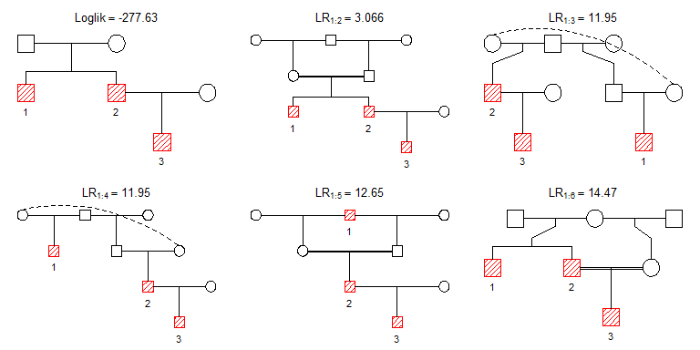
The most likely results this time are shown below:
plot(res2, top = 6)
We see that the same pedigree “wins”, but some esoteric alternatives have appeared among the runners-up.
extraArguably the most important parameter to reconstruct()
is extra, which controls the size of the pedigrees to
consider. It can be either a nonnegative integer, or the word “parents”.
If an integer, it sets the maximum number of extra members used to
connect the original individuals. (The final pedigrees may contain
further extras still, since missing parents are added at the end.)
If extra = "parents", a special algorithm is invoked.
First all directed acyclic graphs between the original individuals are
generated, and then parents are added in all possible ways. This is
(currently) the default behaviour, since it avoids setting an ad
hoc number of “extras”. However, it only works well in relatively
small cases.