![]()
![]()
{rgeedim} supports search and download of Google Earth Engine imagery
with Python module geedim by Dugal
Harris. This package provides wrapper functions that make it more
convenient to use geedim from R.
The rgeedim manual describes the R API. See the geedim manual for more information on Python API and command line interface.
By using geedim images larger than the Image.getDownloadURL()
size limit are split and downloaded as separate tiles, then
re-assembled into a single GeoTIFF.
{rgeedim} is available on CRAN, and can be installed as follows:
install.packages("rgeedim")You can install the development version of {rgeedim} using {remotes}:
if (!require("remotes")) install.packages("remotes")
remotes::install_github("brownag/rgeedim")You will need Python 3 with the geedim module installed
to use {rgeedim}.
pipYou can install geedim with pip, for
example:
python -m pip install geedimThis shell command assumes you have a Python 3 executable named (or
aliased) as python on your PATH, or the command is being
called from within an active Python virtual environment.
If you do not have a Python environment set up, an option that
{reticulate} provides is reticulate::install_miniconda().
Once you install Miniconda, you can install packages into a conda
environment such as "r-reticulate" (default). Customize the
envname argument to create or add to a specific
environment.
reticulate::install_miniconda()
reticulate::py_install("geedim")If using Python within RStudio for the first time, you may need to set your default interpreter in Tools >> Global Options… >> Python.
If you have trouble compiling dependency packages on Windows, you can
take advantage of the unofficial pip wheels (binaries)
prepared by by Christoph Gohlke:
https://www.lfd.uci.edu/~gohlke/pythonlibs/. Note
the name of the package and the specific version of Python you are
installing for. Download the desired package/version and then call
pip install your-package.whl.
This example shows how to extract a Google Earth Engine asset by name
for an arbitrary extent. The coordinates of the bounding box are
expressed in WGS84 decimal degrees ("OGC:CRS84").
library(rgeedim)
#> rgeedim v0.2.0 -- using geedim 1.7.0 w/ earthengine-api 0.1.334
If this is your first time using any Google Earth Engine tools,
authenticate with gd_authenticate(). You can pass arguments
to use several different authorization methods. Perhaps the easiest to
use is auth_mode="notebook" in that does not rely on an
existing GOOGLE_APPLICATION_CREDENTIALS file nor an
installation of the gcloud CLI tools. However, the other
options are better for non-interactive use.
gd_authenticate(auth_mode = "notebook")In each R session you will need to initialize the Earth Engine library
gd_initialize()gd_bbox() is a simple function for specifying extents to
{rgeedim} functions like gd_download():
r <- gd_bbox(
  xmin = -120.6032,
  xmax = -120.5377,
  ymin = 38.0807,
  ymax = 38.1043
)
We will download the US NED CHILI (Continuous Heat-Insolation Load Index) https://developers.google.com/earth-engine/datasets/catalog/CSP_ERGo_1_0_US_CHILI. We specify an equal-area coordinate reference system (NAD83 Albers), bilinear resampling, and a resolution of 10 meters.
res <- 'CSP/ERGo/1_0/US/CHILI' |>
          gd_image_from_id() |>
          gd_download(
            filename = 'image.tif',
            region = r,
            crs = "EPSG:5070",
            resampling = "bilinear",
            scale = 10, # scale=10: request ~10m resolution
            overwrite = TRUE,
            silent = FALSE
          )
We can inspect our results with {terra}. The resulting GeoTIFF has
two layers, "constant" and "FILL_MASK". The
former contains the data, and the latter contains a mask reflecting data
availability (value = 1 where data are available).
library(terra)
#> terra 1.6.47

f <- rast(res)
f
#> class       : SpatRaster
#> dimensions  : 402, 618, 2  (nrow, ncol, nlyr)
#> resolution  : 10, 10  (x, y)
#> extent      : -2113880, -2107700, 1945580, 1949600  (xmin, xmax, ymin, ymax)
#> coord. ref. : NAD83 / Conus Albers (EPSG:5070)
#> source      : image.tif
#> names       : constant, FILL_MASK

plot(f[[1]])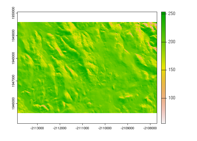
This example demonstrates the download of a section of the USGS NED seamless 10m grid. This DEM is processed with {terra} to calculate some terrain derivatives (slope, aspect) and a hillshade.
library(rgeedim)
library(terra)

gd_initialize()

b <- gd_bbox(
  xmin = -120.296,
  xmax = -120.227,
  ymin = 37.9824,
  ymax = 38.0071
)

## hillshade example
# download 10m NED DEM in AEA
x <- "USGS/NED" |>
  gd_image_from_id() |>
  gd_download(
    region = b,
    scale = 10,
    crs = "EPSG:5070",
    resampling = "bilinear",
    filename = "image.tif",
    overwrite = TRUE,
    silent = FALSE
  )
dem <- rast(x)$elevation

# calculate slope, aspect, and hillshade with terra
slp <- terrain(dem, "slope", unit = "radians")
asp <- terrain(dem, "aspect", unit = "radians")
hsd <- shade(slp, asp)

# compare elevation v.s. hillshade
plot(c(dem, hillshade = hsd))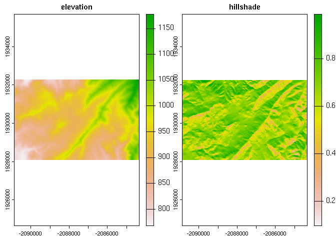
This example demonstrates how to access the 1m LiDAR data from USGS.
A key step in this process is the use of gd_composite() to
resample the component images prior to download.
library(rgeedim)
library(terra)

# search and download from USGS 1m lidar data collection
gd_initialize()

# wkt->SpatExtent
b <- 'POLYGON((-121.355 37.56,-121.355 37.555,
          -121.35 37.555,-121.35 37.56,
          -121.355 37.56))' |>
  vect(crs = "OGC:CRS84")
r <- gd_region(b)

# note that resampling is done on the images as part of compositing/before download
x <- "USGS/3DEP/1m" |>
  gd_collection_from_name() |>
  gd_search(region = r) |>
  gd_composite(resampling = "bilinear") |>
  gd_download(region = r,
              crs = "EPSG:5070",
              scale = 1,
              filename = "image.tif",
              overwrite = TRUE,
              silent = FALSE) |>
  rast()

# inspect
plot(terra::terrain(x$elevation))
plot(project(b, x), add = TRUE)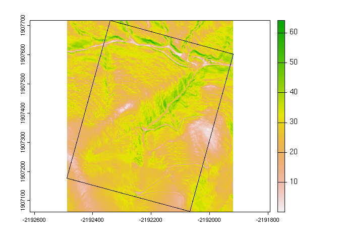
This example demonstrates download of a Landsat-7 cloud/shadow-free
composite image. A collection is created from the USGS Landsat 7 Level
2, Collection 2, Tier 1. This example is based on a tutorial
in the geedim manual.
library(rgeedim)
library(terra)

gd_initialize()

b <- gd_bbox(
  xmin = -120.296,
  xmax = -120.227,
  ymin = 37.9824,
  ymax = 38.0071
)

## landsat example
# search collection for date range and minimum data fill (85%)
x <- 'LANDSAT/LE07/C02/T1_L2' |>
  gd_collection_from_name() |>
  gd_search(
    start_date = '2020-11-01',
    end_date = '2021-02-28',
    region = b,
    cloudless_portion = 85
  )

# inspect individual image metadata in the collection
gd_properties(x)
#>                                            id                date  fill
#> 1 LANDSAT/LE07/C02/T1_L2/LE07_043034_20201130 2020-11-29 16:00:00 86.41
#> 2 LANDSAT/LE07/C02/T1_L2/LE07_043034_20210101 2020-12-31 16:00:00 86.85
#> 3 LANDSAT/LE07/C02/T1_L2/LE07_043034_20210117 2021-01-16 16:00:00 86.05
#> 4 LANDSAT/LE07/C02/T1_L2/LE07_043034_20210218 2021-02-17 16:00:00 85.66
#>   cloudless grmse    saa   sea
#> 1     99.98  4.92 151.45 25.21
#> 2     98.89  4.79 148.07 22.47
#> 3     99.93  5.44 145.16 23.71
#> 4     99.91  5.73 138.46 30.91

# download a single image
y <- gd_properties(x)$id[1] |>
  gd_image_from_id() |>
  gd_download(
    filename = "image.tif",
    region = b,
    scale = 30,
    crs = 'EPSG:5070',
    dtype = 'uint16',
    overwrite = TRUE,
    silent = FALSE
  )
plot(rast(y)[[1:4]])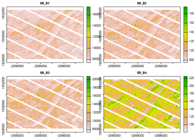
# create composite landsat image near December 1st, 2020 and download
# using q-mosaic method.
z <- x |>
  gd_composite(
    method = "q-mosaic",
    date = '2020-12-01'
  ) |>
  gd_download(
    filename = "image.tif",
    region = b,
    scale = 30,
    crs = 'EPSG:5070',
    dtype = 'uint16',
    overwrite = TRUE,
    silent = FALSE
  )
plot(rast(z)[[1:4]])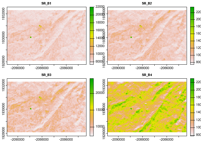
The "q-mosaic" method produces a composite largely free
of artifacts; this is because it prioritizes pixels with higher distance
from clouds.