The {sherlock} R package provides powerful graphical
displays and statistical tools to aid structured problem solving and
diagnosis. The functions of the package are especially useful for
applying the process of elimination as a problem diagnosis technique.
{sherlock} was designed to seamlessly work with the
tidyverse set of packages.
“That is to say, nature’s laws are causal; they reveal themselves by comparison and difference, and they operate at every multi-variate space-time point” - Edward Tufte
You can install the development version of sherlock from
GitHub with:
# install.packages("devtools")
devtools::install_github("gaborszabo11/sherlock")While the package is currently under development, quite a few functions are already available and ready to be used. Available functions are as follows:
draw_multivari_plot()
draw_categorical_scatterplot()
draw_youden_plot()
draw_small_multiples_line_plot()
draw_cartesian_small_multiples()
draw_polar_small_multiples()
draw_interaction_plot()
draw_process_behavior_chart()
draw_timeseries_scatterplot()
load_file()
save_analysis()
normalize_observations()
theme_sherlock()
scale_color_sherlock()
scale_fill_sherlock()
draw_horizontal_reference_line()
draw_vertical_reference_line()
Here are a few examples:
# Loading libraries
library(sherlock)
library(ggh4x)
#> Loading required package: ggplot2
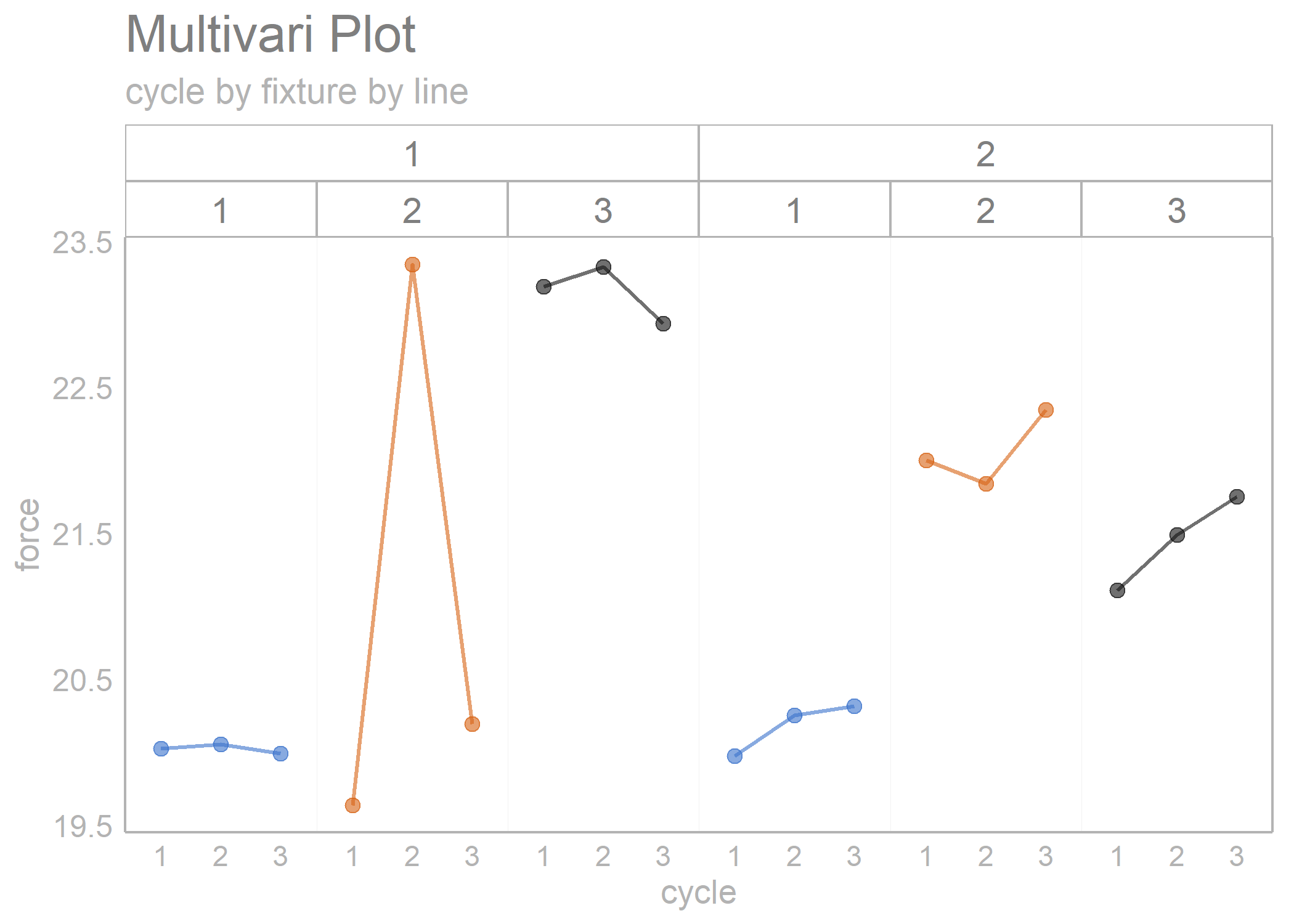
multi_vari_data %>%
draw_multivari_plot(response = force,
factor_1 = cycle,
factor_2 = fixture,
factor_3 = line)
library(sherlock)
library(ggh4x)

multi_vari_data_2 %>%
  draw_multivari_plot(response = Length,
                      factor_1 = Part,
                      factor_2 = Operator, plot_means = TRUE)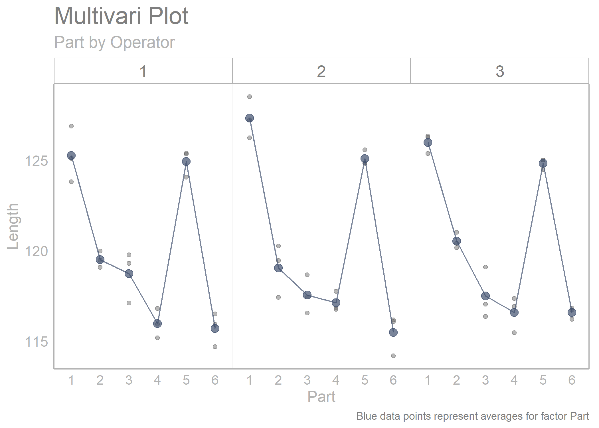
library(sherlock)
library(dplyr)
#>
#> Attaching package: 'dplyr'
#> The following objects are masked from 'package:stats':
#>
#>     filter, lag
#> The following objects are masked from 'package:base':
#>
#>     intersect, setdiff, setequal, union

polar_small_multiples_data %>%
  filter(Mold_Cavity_Number %in% c(4, 6)) %>%
  draw_polar_small_multiples(angular_axis   = ID_Measurement_Angle,
                             x_y_coord_axis = ID_2,
                             grouping_var   = Tip_Bottom,
                             faceting_var_1 = Mold_Cavity_Number,
                             point_size     = 0.5,
                             connect_with_lines = TRUE,
                             label_text_size = 7)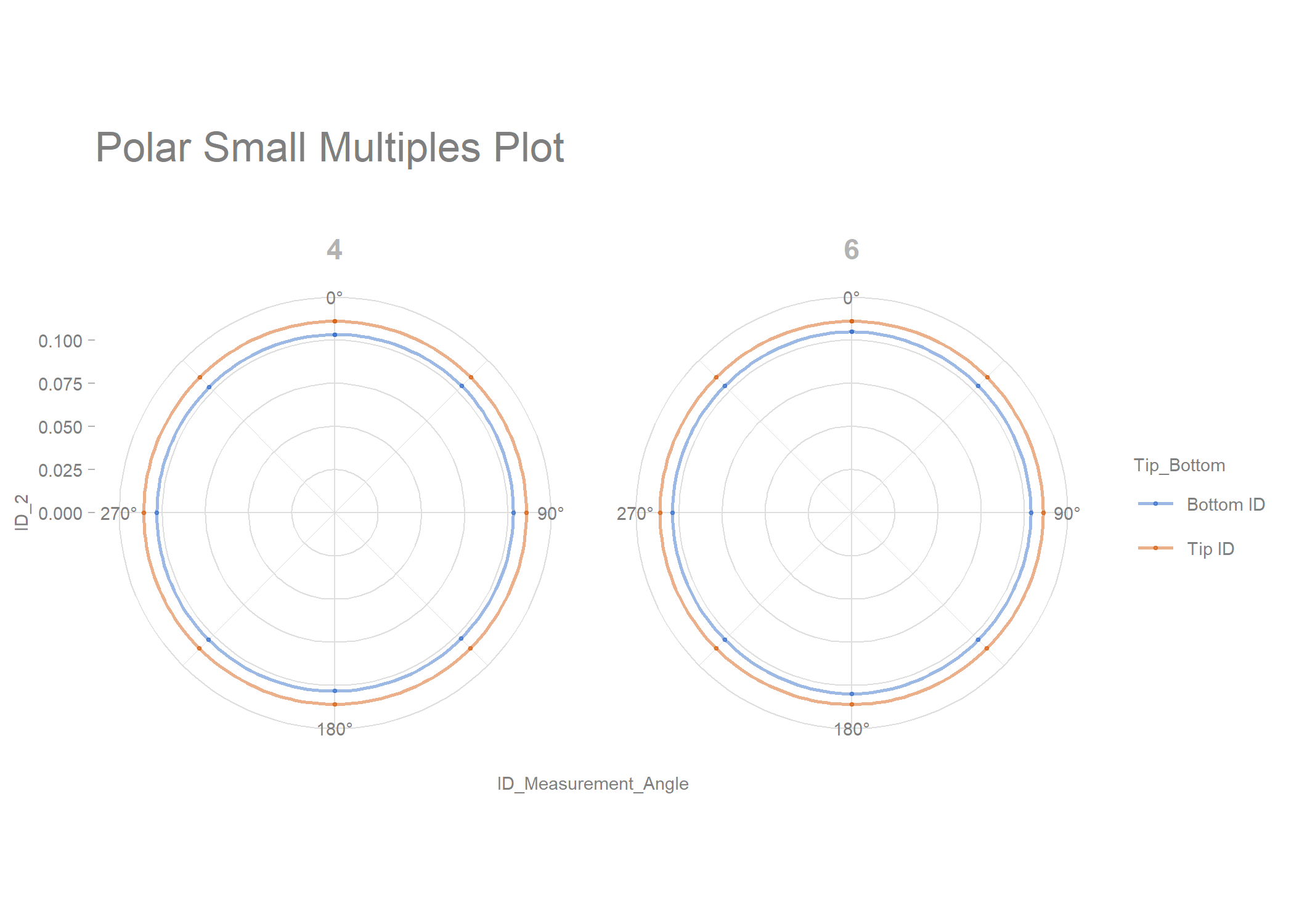
library(sherlock)
library(dplyr)
library(ggh4x)

polar_small_multiples_data %>%
  filter(ID_Measurement_Angle %in% c(0, 45, 90, 135)) %>%
  normalize_observations(response = ID, grouping_var = Tip_Bottom, ref_values = c(0.2075, 0.2225)) %>%
  draw_multivari_plot(response    = ID_normalized,
                      factor_1    = ID_Measurement_Angle,
                      factor_2    = Mold_Cavity_Number,
                      factor_3    = Tip_Bottom,
                      x_axis_text = 6) +
  draw_horizontal_reference_line(reference_line = 0)
#> Joining, by = "Tip_Bottom"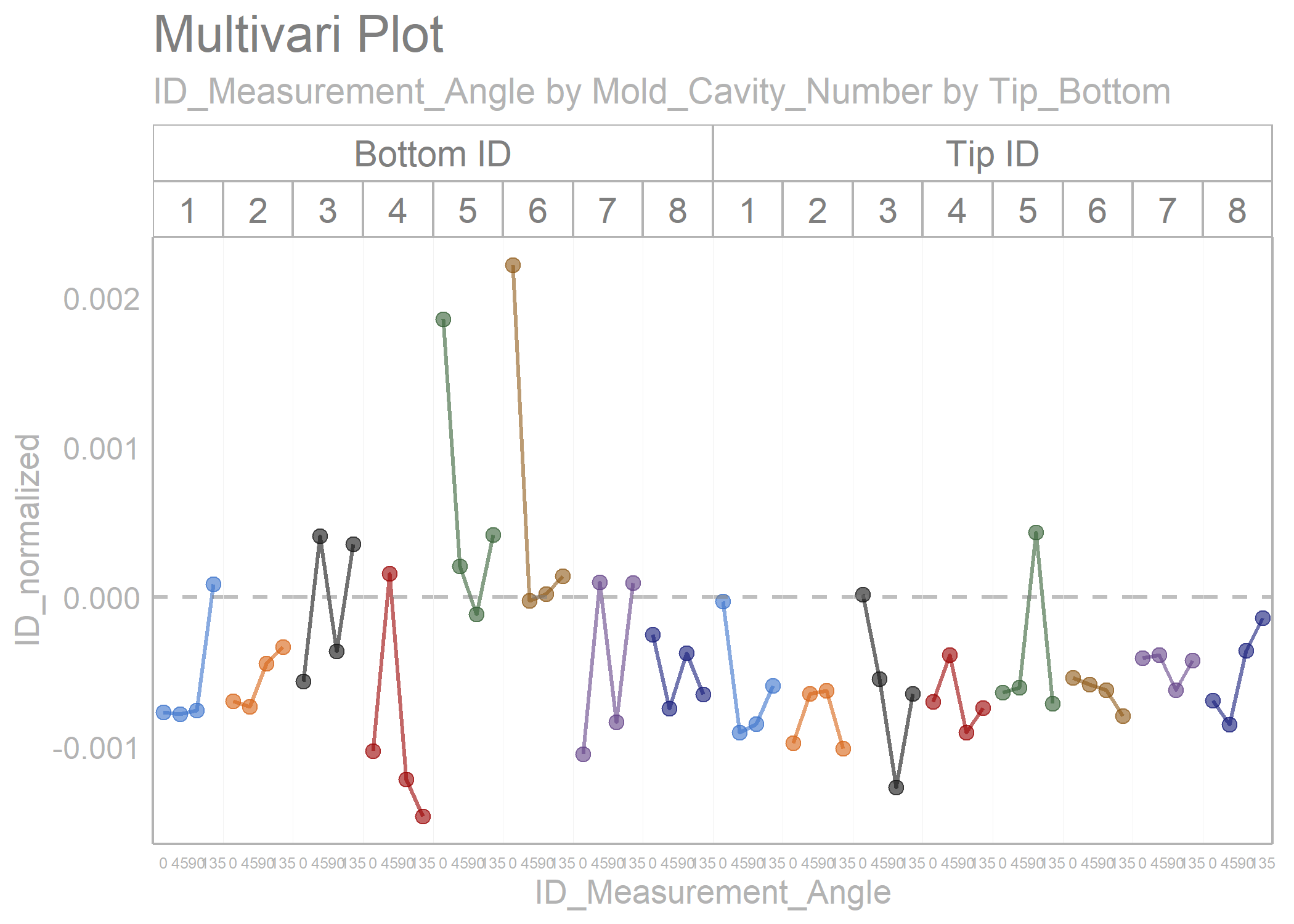
youden_plot_data_2 %>%
  draw_youden_plot(x_axis_var  = gage_1,
                   y_axis_var  = gage_2,
                   median_line = TRUE)
#> Smoothing formula not specified. Using: y ~ x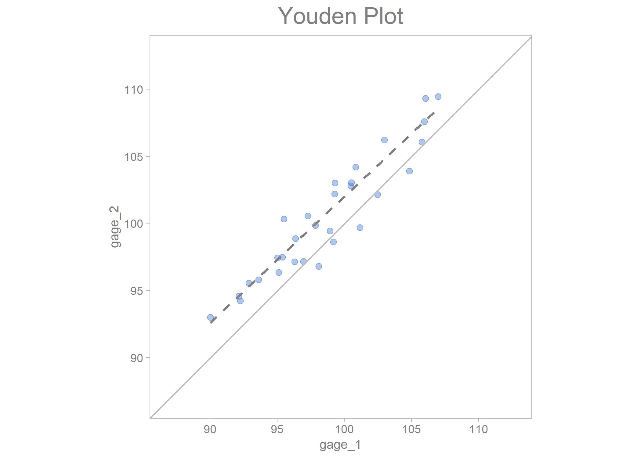
youden_plot_data %>%
  draw_youden_plot(x_axis_var   = measurement_1,
                   y_axis_var   = measurement_2,
                   grouping_var = location,
                   x_axis_label = "Trial 1",
                   y_axis_label = "Trial 2")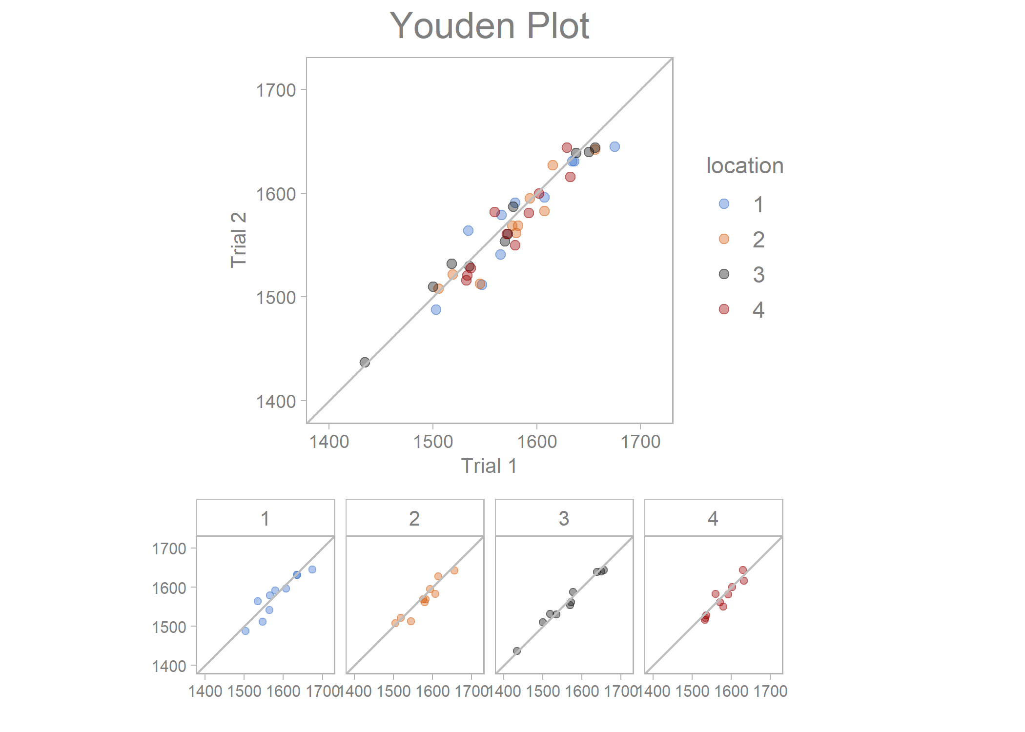
timeseries_scatterplot_data %>%
  draw_timeseries_scatterplot(y_var = y,
                              grouping_var_1 = date,
                              grouping_var_2 = cavity,
                              faceting       = TRUE,
                              limits         = TRUE,
                              alpha          = 0.15,
                              line_size      = 0.5,
                              x_axis_text    = 7,
                              interactive    = FALSE)
#> Joining, by = c("date", "cavity")
#> Warning: Removed 6 rows containing missing values (geom_point).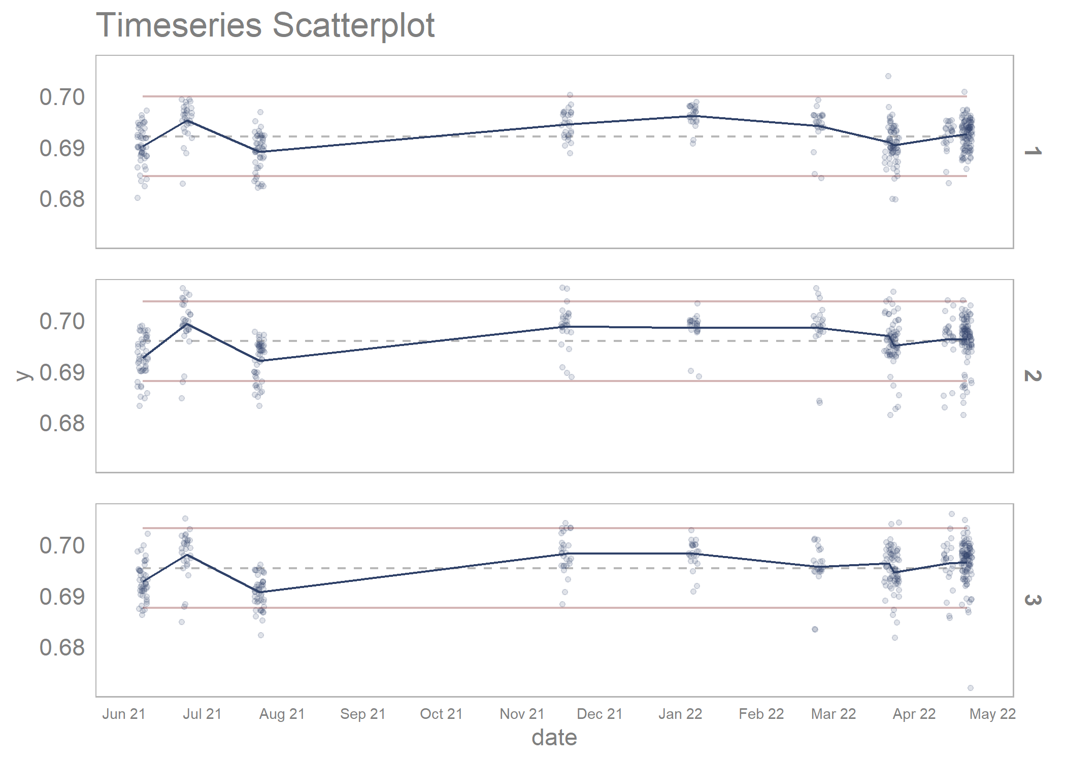
Diagnosing Performance and Reliability, David Hartshorne and The New Science of Fixing Things, 2019
Statistical Engineering - An Algorithm for Reducing Variation in Manufacturing Processes, Stefan H. Steiner and Jock MacKay, 2005