
Functions to connect the widely used Storm Water Management Model (SWMM) of the United States Environmental Protection Agency (US EPA) to R with currently two main goals: (1) Run a SWMM simulation from R and (2) provide fast access to simulation results, i.e. SWMM’s binary ‘.out’-files. High performance is achieved with help of Rcpp. Additionally, reading SWMM’s ‘.inp’ and ‘.rpt’ files is supported to glance model structures and to get direct access to simulation summaries.
Installation is easy thanks to CRAN:
install.packages("swmmr")You can install the dev version from github with:
# install.packages("remotes")
remotes::install_github("dleutnant/swmmr")This is a basic example which shows you how to work with the package. We use the example shipped with the SWMM5 executable.
library(swmmr)
library(purrr) # to conveniently work with list objects

# set path to inp
# If your operating system is Windows, the Example model files are usually
# located at "C:\Users\your user name\Documents\EPA SWMM Projects\Examples".
# For convenience the Example1.inp model is also included in the swmmr package.
inp_path <- system.file("extdata", "Example1.inp", package = "swmmr", mustWork = TRUE)

# glance model structure, the result is a list of data.frames with SWMM sections
inp <- read_inp(x = inp_path)

# show swmm model summary
summary(inp)
#>
#> ** summary of swmm model structure **
#> infiltration   :     horton
#> flow_units     :        cfs
#> flow_routing   :    kinwave
#> start_date     : 01/01/1998
#> end_date       : 01/02/1998
#> raingages      :          1
#> subcatchments  :          8
#> aquifers       :          0
#> snowpacks      :          0
#> junctions      :         13
#> outfalls       :          1
#> dividers       :          0
#> storage        :          0
#> conduits       :         13
#> pumps          :          0
#> orifices       :          0
#> weirs          :          0
#> outlets        :          0
#> controls       :          0
#> pollutants     :          2
#> landuses       :          2
#> lid_controls   :          0
#> treatment      :          0
#> *************************************

# for example, inspect section subcatchments
inp$subcatchments
#> # A tibble: 8 x 9
#>   Name  `Rain Gage` Outlet  Area Perc_Imperv Width Perc_Slope CurbLen Snowpack
#>   <chr> <chr>       <chr>  <int>       <int> <int>      <dbl>   <int> <lgl>
#> 1 1     RG1         9         10          50   500       0.01       0 NA
#> 2 2     RG1         10        10          50   500       0.01       0 NA
#> 3 3     RG1         13         5          50   500       0.01       0 NA
#> 4 4     RG1         22         5          50   500       0.01       0 NA
#> 5 5     RG1         15        15          50   500       0.01       0 NA
#> 6 6     RG1         23        12          10   500       0.01       0 NA
#> 7 7     RG1         19         4          10   500       0.01       0 NA
#> 8 8     RG1         18        10          10   500       0.01       0 NA

# run a simulation
# the result is a named list of paths, directing
# to the inp, rpt and out-file, respectively.
files <- run_swmm(inp = inp_path)
#> arguments 'minimized' and 'invisible' are for Windows only

# we can now read model results from the binary output:
# here, we focus on the system variable (iType = 3) from which we pull
# total rainfall (in/hr or mm/hr) and total runoff (flow units) (vIndex = c(1,4)).
results <- read_out(files$out, iType = 3, vIndex = c(1, 4))

# results is a list object containing two time series
str(results, max.level = 2)
#> List of 1
#>  $ system_variable:List of 2
#>   ..$ total_rainfall:An 'xts' object on 1998-01-01 01:00:00/1998-01-02 12:00:00 containing:
#>   Data: num [1:36, 1] 0.25 0.5 0.8 0.4 0.1 ...
#>   Indexed by objects of class: [POSIXct,POSIXt] TZ: GMT
#>   xts Attributes:
#>  NULL
#>   ..$ total_runoff  :An 'xts' object on 1998-01-01 01:00:00/1998-01-02 12:00:00 containing:
#>   Data: num [1:36, 1] 0 6.22 13.03 24.25 14.17 ...
#>   Indexed by objects of class: [POSIXct,POSIXt] TZ: GMT
#>   xts Attributes:
#>  NULL

# basic summary
results[[1]] %>% invoke(merge, .) %>% summary
#>      Index                     total_rainfall     total_runoff
#>  Min.   :1998-01-01 01:00:00   Min.   :0.00000   Min.   : 0.0000
#>  1st Qu.:1998-01-01 09:45:00   1st Qu.:0.00000   1st Qu.: 0.0000
#>  Median :1998-01-01 18:30:00   Median :0.00000   Median : 0.0000
#>  Mean   :1998-01-01 18:30:00   Mean   :0.07361   Mean   : 2.1592
#>  3rd Qu.:1998-01-02 03:15:00   3rd Qu.:0.00000   3rd Qu.: 0.1033
#>  Max.   :1998-01-02 12:00:00   Max.   :0.80000   Max.   :24.2530

# basic plotting
results[[1]] %>% imap( ~ plot(.x, main = .y))
#> $total_rainfall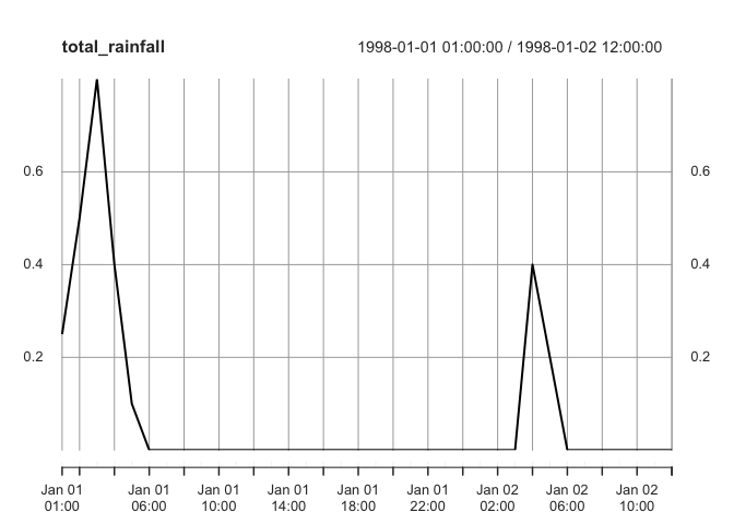
#>
#> $total_runoff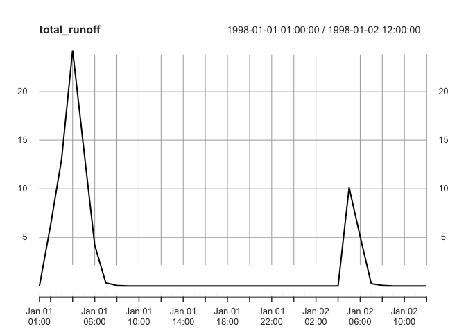
# We also might be interested in the report file:
# use read_rpt to get is a list of data.frames with SWMM summary sections
report <- read_rpt(files$rpt)

# glance available summaries
summary(report)
#>                                  Length Class  Mode
#> analysis_options                 2      tbl_df list
#> runoff_quantity_continuity       3      tbl_df list
#> runoff_quality_continuity        3      tbl_df list
#> flow_routing_continuity          3      tbl_df list
#> quality_routing_continuity       3      tbl_df list
#> highest_flow_instability_indexes 2      tbl_df list
#> routing_time_step_summary        2      tbl_df list
#> subcatchment_runoff_summary      9      tbl_df list
#> subcatchment_washoff_summary     3      tbl_df list
#> node_depth_summary               8      tbl_df list
#> node_inflow_summary              9      tbl_df list
#> node_flooding_summary            7      tbl_df list
#> outfall_loading_summary          7      tbl_df list
#> link_flow_summary                8      tbl_df list
#> conduit_surcharge_summary        6      tbl_df list
#> link_pollutant_load_summary      3      tbl_df list
#> analysis_info                    1      tbl_df list

# convenient access to summaries through list structure
report$subcatchment_runoff_summary
#> # A tibble: 8 x 9
#>   Subcatchment Total_Precip Total_Runon Total_Evap Total_Infil Total_Runoff_De…
#>   <chr>               <dbl>       <dbl>      <dbl>       <dbl>            <dbl>
#> 1 1                    2.65           0          0        1.16             1.32
#> 2 2                    2.65           0          0        1.21             1.32
#> 3 3                    2.65           0          0        1.16             1.32
#> 4 4                    2.65           0          0        1.16             1.32
#> 5 5                    2.65           0          0        1.24             1.31
#> 6 6                    2.65           0          0        2.27             0.26
#> 7 7                    2.65           0          0        2.14             0.26
#> 8 8                    2.65           0          0        2.25             0.26
#> # … with 3 more variables: Total_Runoff_Volume <dbl>, Total_Peak_Runoff <dbl>,
#> # Total_Runoff_Coeff <chr>With help of packages ‘ggplot2’ and ‘sf’ we can easily plot entire
swmm models. Note that ggplot2 (>= 2.2.1.9000) is required, which
provides the geometric object geom_sf().
library(ggplot2)

# initially, we convert the objects to be plotted as sf objects:
# here: subcatchments, links, junctions, raingages
sub_sf <- subcatchments_to_sf(inp)
lin_sf <- links_to_sf(inp)
jun_sf <- junctions_to_sf(inp)
rg_sf <- raingages_to_sf(inp)

# calculate coordinates (centroid of subcatchment) for label position
lab_coord <- sub_sf %>%
  sf::st_centroid() %>%
  sf::st_coordinates() %>%
  tibble::as_tibble()
#> Warning in st_centroid.sf(.): st_centroid assumes attributes are constant over
#> geometries of x

# raingage label
lab_rg_coord <- rg_sf %>%
  {sf::st_coordinates(.) + 500} %>% # add offset
  tibble::as_tibble()

# add coordinates to sf tbl
sub_sf <- dplyr::bind_cols(sub_sf, lab_coord)
rg_sf <- dplyr::bind_cols(rg_sf, lab_rg_coord)

# create the plot
ggplot() +
  # first plot the subcatchment and colour continously by Area
  geom_sf(data = sub_sf, aes(fill = Area)) +
  # label by subcatchments by name
  geom_label(data = sub_sf, aes(X, Y, label = Name), alpha = 0.5, size = 3) +
  # add links and highlight Geom1
  geom_sf(data = lin_sf, aes(colour = Geom1), size = 2) +
  # add junctions
  geom_sf(data = jun_sf, aes(size = Elevation), colour = "darkgrey") +
  # finally show location of raingage
  geom_sf(data = rg_sf, shape = 10) +
  # label raingage
  geom_label(data = rg_sf, aes(X, Y, label = Name), alpha = 0.5, size = 3) +
  # change scales
  scale_fill_viridis_c() +
  scale_colour_viridis_c(direction = -1) +
  # change theme
  theme_linedraw() +
  theme(panel.grid.major = element_line(colour = "white")) +
  # add labels
  labs(title = "SWMM model Example1",
       subtitle = "customized visualization")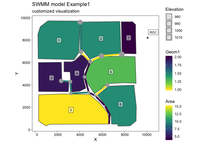
With the release of swmmr 0.9.0, the latest
contributions and other code that will appear in the next CRAN release
is contained in the master
branch. Thus, contributing to this package is easy. Just send a simple
pull
request. Your PR should pass R CMD check --as-cran,
which will also be checked by
Travis CI when the
PR is submitted.
Please note that this project is released with a Contributor Code of Conduct. By participating in this project you agree to abide by its terms.
This package has been mainly developed in the course of the project STBMOD, carried out at the Institute for Infrastructure, Water, Resources, Environment (IWARU) of the Muenster University of Applied Sciences. The project was funded by the German Federal Ministry of Education and Research (BMBF, FKZ 03FH033PX2).
The development of the R package was inspired by the work of Peter Steinberg. Also, it benefits from the Interface Guide of SWMM.
To cite ‘swmmr’ in publications, please use:
Dominik Leutnant, Anneke Döring & Mathias Uhl (2019). swmmr - an R package to interface SWMM Urban Water Journal DOI: 10.1080/1573062X.2019.1611889
A BibTeX entry for LaTeX users is
@Article{, author = {Dominik Leutnant and Anneke Döring and Mathias Uhl}, title = {swmmr - an R package to interface SWMM}, journal = {Urban Water Journal}, volume = {16}, number = {1}, pages = {68-76}, year = {2019}, publisher = {Taylor & Francis}, doi = {10.1080/1573062X.2019.1611889}, url = {https://doi.org/10.1080/1573062X.2019.1611889}, eprint = {https://doi.org/10.1080/1573062X.2019.1611889}, }