The goal of tehtuner is to implement methods to fit
models to detect and model treatment effect heterogeneity (TEH) while
controlling the Type-I error of falsely detecting a differential effect
when the conditional average treatment effect is uniform across the
study population.
Currently tehtuner supports Virtual Twins models (Foster
et al., 2011) for detecting TEH.
Virtual Twins is a two-step approach to detecting differential treatment effects. Subjects’ conditional average treatment effects (CATEs) are first estimated in Step 1 using a flexible model. Then, a simple and interpretable model is fit in Step 2 to model these estimated CATEs as a function of the covariates.
The Step 2 model is dependent on some tuning parameter. This parameter is selected to control the Type-I error rate by permuting the data under the null hypothesis of a constant treatment effect and identifying the minimal null penalty parameter (MNPP), which is the smallest penalty parameter that yields a Step 2 model with no covariate effects. The \(1-\alpha\) quantile of the distribution of is then used to fit the Step 2 model on the original data. In dong so, the Type-I error rate is controlled to be \(\alpha\).
tehtuner is not currently available on CRAN.
You can download the development version from GitHub with:
# install.packages("devtools")
devtools::install_github("jackmwolf/tehtuner")We consider simulated data from a small clinical trial with 200 subjects. Each subject has 10 measured covaraites, 8 continuous and 2 binary. We are interested in estimating and understanding the CATE through Virtual Twins.
library(tehtuner)
data("tehtuner_example")
tehtuner_example %>%
  head %>%
kbl(booktabs = TRUE, digits = 2, format = "markdown")| Trt | Y | V1 | V2 | V3 | V4 | V5 | V6 | V7 | V8 | V9 | V10 |
|---|---|---|---|---|---|---|---|---|---|---|---|
| 0 | 0.56 | -1.41 | -3.87 | 0.22 | 1.77 | -1.43 | -0.14 | -1.29 | 2.15 | 1 | 1 |
| 0 | -2.64 | -0.68 | -3.50 | -1.01 | 1.30 | -3.62 | -2.52 | -2.71 | 1.77 | 1 | 1 |
| 0 | 3.04 | -4.34 | -5.76 | -2.25 | 1.12 | -3.68 | -1.21 | -2.07 | 1.65 | 1 | 1 |
| 0 | 0.22 | 0.59 | -3.87 | -0.68 | 0.81 | -2.89 | -1.47 | -1.83 | 1.70 | 1 | 1 |
| 0 | -0.97 | -1.94 | -2.59 | -0.29 | 0.23 | -3.19 | -1.93 | -1.69 | 2.18 | 0 | 0 |
| 0 | -3.61 | -0.32 | -2.58 | 0.36 | 1.94 | -2.35 | -3.01 | -1.69 | 2.85 | 0 | 0 |
We will consider a Virtual Twins model using a random forest to estimate the CATEs in Step 1 and then fitting a regression tree on the estimated CATEs in Step 2 with the Type-I error rate set at \(\alpha = 0.2\).
set.seed(100)
vt_cate <- tunevt(
  data = tehtuner_example, Y = "Y", Trt = "Trt", step1 = "randomforest",
  step2 = "rtree", alpha0 = 0.2, p_reps = 100, ntree = 50
)
The fitted Step 2 model can be accessed via $vtmod. In
this case, as we used a regression tree in Step 2, our final model model
is of class rpart.
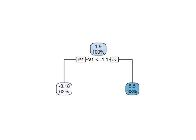
vt_cate$vtmod
#> n= 200
#>
#> node), split, n, deviance, yval
#>       * denotes terminal node
#>
#> 1) root 200 4282.543  1.9449220
#>   2) V1< -1.081597 125 1418.895 -0.1780733 *
#>   3) V1>=-1.081597 75 1361.278  5.4832470 *

rpart.plot::rpart.plot(vt_cate$vtmod)
The fitted model for the CATE includes a covariate (V1),
so we would conclude that there is treatment effect heterogeneity at the
20% level. (We note that the true data generating mechanism (\(Y_i = h(X_i) + T_i g(X_i)\)) included an
interaction between the treatment and whether \(V_1\) was above its true mean [sample mean
-1.34] with \(g(X_i) = c +
4I(V_{1i}>\mu_1)+4V_{9i}\). So, the procedure did not make a
Type-I error and correctly detected a covariate driving this
heterogeneity.)
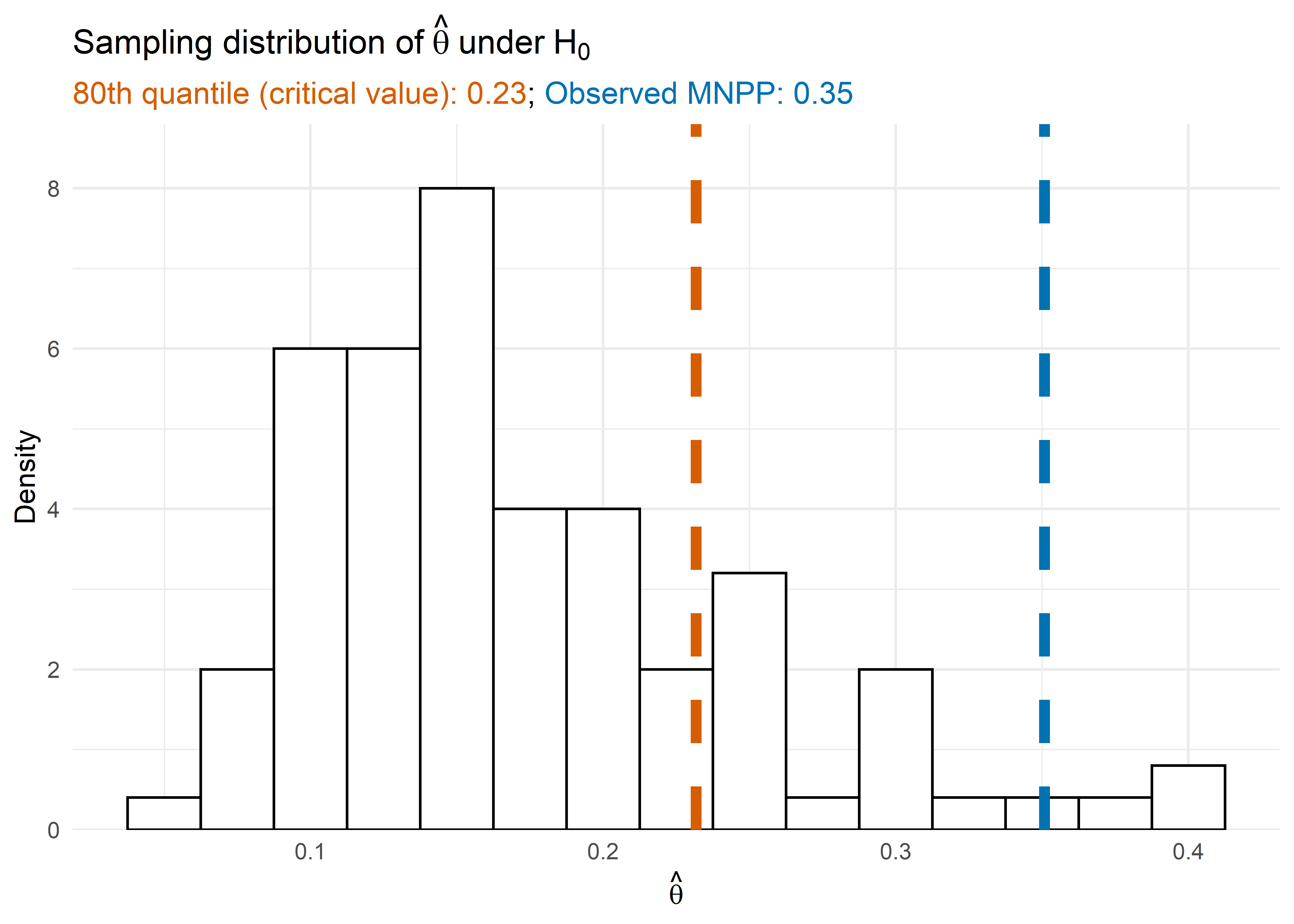
We can also look at the null distribution of the MNPP through
vt_cate$theta_null. The 80th quantile of \(\hat\theta\) under the null hypothesis
is
quantile(vt_cate$theta_null, 0.8)
#>       80%
#> 0.2317442
while the MNPP of our observed data is
vt_cate$mnpp
#> [1] 0.3508124
The procedure fit the Step 2 model using the 80th quantile of the null distribution which resulted in a model that included covariates since the MNPP was above the 80th quantile.

Foster, J. C., Taylor, J. M., & Ruberg, S. J. (2011). Subgroup identification from randomized clinical trial data. Statistics in Medicine, 30(24), 2867–2880. https://doi.org/10.1002/sim.4322
Wolf, J. M., Koopmeiners, J. S., & Vock, D. M. (2022). A permutation procedure to detect heterogeneous treatment effects in randomized clinical trials while controlling the type-I error rate. Clinical Trials 19(5). https://doi.org/10.1177/17407745221095855