![]()

The goal of rFIA is to increase the accessibility and
use of the USFS Forest Inventory and Analysis (FIA) Database by
providing a user-friendly, open source platform to easily query and
analyze FIA Data. Designed to accommodate a wide range of potential user
objectives, rFIA simplifies the estimation of forest
variables from the FIA Database and allows all R users (experts and
newcomers alike) to unlock the flexibility and potential inherent to the
Enhanced FIA design.
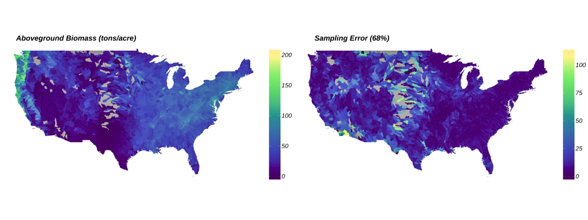
Specifically, rFIA improves accessibility to the
spatio-temporal estimation capacity of the FIA Database by producing
space-time indexed summaries of forest variables within user-defined
population boundaries. Direct integration with other popular R packages
(e.g., dplyr, sp, and sf) facilitates efficient space-time query and
data summary, and supports common data representations and API design.
The package implements design-based estimation procedures outlined by
Bechtold & Patterson (2005), and has been validated against
estimates and sampling errors produced by EVALIDator. Current
development is focused on the implementation of spatially-enabled
model-assisted estimators to improve population, change, and ratio
estimates.
For more information and example usage of rFIA, check
out our website. To report a bug
or suggest additions to rFIA, please use our active issues
page here on GitHub, or contact Hunter Stanke (lead developer and
maintainer).
To cite rFIA, please refer to
our recent publication in Environmental
Modeling and Software (doi: https://doi.org/10.1016/j.envsoft.2020.104664).
You can install the released version of rFIA from CRAN with:
install.packages("rFIA")Alternatively, you can install the development version from GitHub:
devtools::install_github('hunter-stanke/rFIA')rFIA Function |
Description |
|---|---|
area |
Estimate land area in various classes |
biomass |
Estimate volume, biomass, & carbon stocks of standing trees |
clipFIA |
Spatial & temporal queries for FIA data |
diversity |
Estimate diversity indices (e.g. species diversity) |
dwm |
Estimate volume, biomass, and carbon stocks of down woody material |
getFIA |
Download FIA data, load into R, and optionally save to disk |
growMort |
Estimate recruitment, mortality, and harvest rates |
invasive |
Estimate areal coverage of invasive species |
plotFIA |
Produce static & animated plots of FIA summaries |
readFIA |
Load FIA database into R environment from disk |
seedling |
Estimate seedling abundance (TPA) |
standStruct |
Estimate forest structural stage distributions |
tpa |
Estimate abundance of standing trees (TPA & BAA) |
vitalRates |
Estimate live tree growth rates |
writeFIA |
Write in-memory FIA Database to disk |
The first step to using rFIA is to download subsets of
the FIA Database. The easiest way to accomplish this is using
getFIA. Using one line of code, you can download state
subsets of the FIA Database, load data into your R environment, and
optionally save those data to a local directory for future use!
## Download the state subset or Connecticut (requires an internet connection)
# All data acquired from FIA Datamart: https://apps.fs.usda.gov/fia/datamart/datamart.html
ct <- getFIA(states = 'CT', dir = '/path/to/save/data')
By default, getFIA only loads the portions of the
database required to produce summaries with other rFIA
functions (common = TRUE). This conserves memory on your
machine and speeds download time. If you would like to download all
available tables for a state, simple specify common = FALSE
in the call to getFIA.
But what if I want to load multiple states worth of FIA data
into R? No problem! Simply specify mutiple state abbreviations
in the states argument of getFIA
(e.g. states = c('MI', 'IN', 'WI', 'IL')), and all state
subsets will be downloaded and merged into a single
FIA.Database object. This will allow you to use other
rFIA functions to produce estimates within polygons which
straddle state boundaries!
Note: given the massive size of the full FIA Database, users are cautioned to only download the subsets containing their region of interest.
If you have previously downloaded FIA data would simply like
to load into R from a local directory, use
readFIA:
## Load FIA Data from a local directory
db <- readFIA('/path/to/your/directory/')Now that you have loaded your FIA data into R, it’s time to put it to
work. Let’s explore the basic functionality of rFIA with
tpa, a function to compute tree abundance estimates (TPA,
BAA, & relative abundance) from FIA data, and fiaRI, a
subset of the FIA Database for Rhode Island including inventories from
2013-2018.
Estimate the abundance of live trees in Rhode Island:
library(rFIA)
## Load the Rhode Island subset of the FIADB (included w/ rFIA)
## NOTE: This object can be produced using getFIA and/or readFIA
data("fiaRI")

## Only estimates for the most recent inventory year
fiaRI_MR <- clipFIA(fiaRI, mostRecent = TRUE) ## subset the most recent data
tpaRI_MR <- tpa(fiaRI_MR)
head(tpaRI_MR)
#> # A tibble: 1 x 8
#>    YEAR   TPA   BAA TPA_SE BAA_SE nPlots_TREE nPlots_AREA     N
#>   <int> <dbl> <dbl>  <dbl>  <dbl>       <int>       <int> <int>
#> 1  2018  427.  122.   6.63   3.06         126         127   199

## All Inventory Years Available (i.e., returns a time series)
tpaRI <- tpa(fiaRI)
head(tpaRI)
#> # A tibble: 5 x 8
#>    YEAR   TPA   BAA TPA_SE BAA_SE nPlots_TREE nPlots_AREA     N
#>   <int> <dbl> <dbl>  <dbl>  <dbl>       <int>       <int> <int>
#> 1  2014  466.  120.   6.73   3.09         121         123   196
#> 2  2015  444.  121.   6.40   3.06         122         124   194
#> 3  2016  450.  123.   6.46   2.94         124         125   197
#> 4  2017  441.  123.   6.66   3.01         124         125   196
#> 5  2018  427.  122.   6.63   3.06         126         127   199
What if I want to group estimates by species? How about by size class?
## Group estimates by species
tpaRI_species <- tpa(fiaRI_MR, bySpecies = TRUE)
head(tpaRI_species, n = 3)
#> # A tibble: 3 x 11
#>    YEAR  SPCD COMMON_NAME        SCIENTIFIC_NAME        TPA    BAA TPA_SE BAA_SE
#>   <int> <int> <chr>              <chr>                <dbl>  <dbl>  <dbl>  <dbl>
#> 1  2018    12 balsam fir         Abies balsamea      0.0873 0.0295  114.   114.
#> 2  2018    43 Atlantic white-ce… Chamaecyparis thyo… 0.247  0.180    59.1   56.0
#> 3  2018    68 eastern redcedar   Juniperus virginia… 1.14   0.138    64.8   67.5
#> # … with 3 more variables: nPlots_TREE <int>, nPlots_AREA <int>, N <int>

## Group estimates by size class
## NOTE: Default 2-inch size classes, but you can make your own using makeClasses()
tpaRI_sizeClass <- tpa(fiaRI_MR, bySizeClass = TRUE)
head(tpaRI_sizeClass, n = 3)
#> # A tibble: 3 x 9
#>    YEAR sizeClass   TPA   BAA TPA_SE BAA_SE nPlots_TREE nPlots_AREA     N
#>   <int>     <dbl> <dbl> <dbl>  <dbl>  <dbl>       <int>       <int> <int>
#> 1  2018         1 188.   3.57  13.0   12.8           76         127   199
#> 2  2018         3  68.6  5.76  15.1   15.8           46         127   199
#> 3  2018         5  46.5  9.06   6.51   6.57         115         127   199

## Group by species and size class, and plot the distribution
##  for the most recent inventory year
tpaRI_spsc <- tpa(fiaRI_MR, bySpecies = TRUE, bySizeClass = TRUE)
plotFIA(tpaRI_spsc, BAA, grp = COMMON_NAME, x = sizeClass,
        plot.title = 'Size-class distributions of BAA by species',
        x.lab = 'Size Class (inches)', text.size = .75,
        n.max = 5) # Only want the top 5 species, try n.max = -5 for bottom 5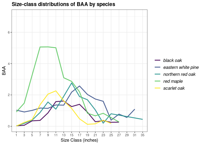
What if I want estimates for a specific type of tree (ex.
greater than 12-inches DBH and in a canopy dominant or subdominant
position) in specific area (ex. growing on mesic sites), and I want to
group by estimates by some variable other than species or size class
(ex. ownsership group)? Easy! Each of these specifications are
described in the FIA Database, and all rFIA functions can
leverage these data to easily implement complex queries!
## grpBy specifies what to group estimates by (just like species and size class above)
## treeDomain describes the trees of interest, in terms of FIA variables
## areaDomain, just like above,describes the land area of interest
tpaRI_own <- tpa(fiaRI_MR,
                     grpBy = OWNGRPCD,
                     treeDomain = DIA > 12 & CCLCD %in% c(1,2),
                     areaDomain = PHYSCLCD %in% c(20:29))
head(tpaRI_own)
#> # A tibble: 2 x 9
#>    YEAR OWNGRPCD   TPA   BAA TPA_SE BAA_SE nPlots_TREE nPlots_AREA     N
#>   <int>    <int> <dbl> <dbl>  <dbl>  <dbl>       <int>       <int> <int>
#> 1  2018       30 0.848  3.57   59.0   59.1           3          38   199
#> 2  2018       40 1.49   3.99   25.7   27.7          12          82   199
What if I want to produce estimates within my own population boundaries (within user-defined spatial zones/polygons)? This is where things get really exciting.
## Load the county boundaries for Rhode Island
data('countiesRI') ## Load your own spatial data from shapefiles using readOGR() (rgdal)

## polys specifies the polygons (zones) where you are interested in producing estimates
## returnSpatial = TRUE indicates that the resulting estimates will be joined with the
##    polygons we specified, thus allowing us to visualize the estimates across space
tpaRI_counties <- tpa(fiaRI_MR, polys = countiesRI, returnSpatial = TRUE)

## NOTE: Any grey polygons below simply means no FIA data was available for that region
plotFIA(tpaRI_counties, BAA) # Plotting method for spatial FIA summaries, also try 'TPA' or 'TPA_PERC'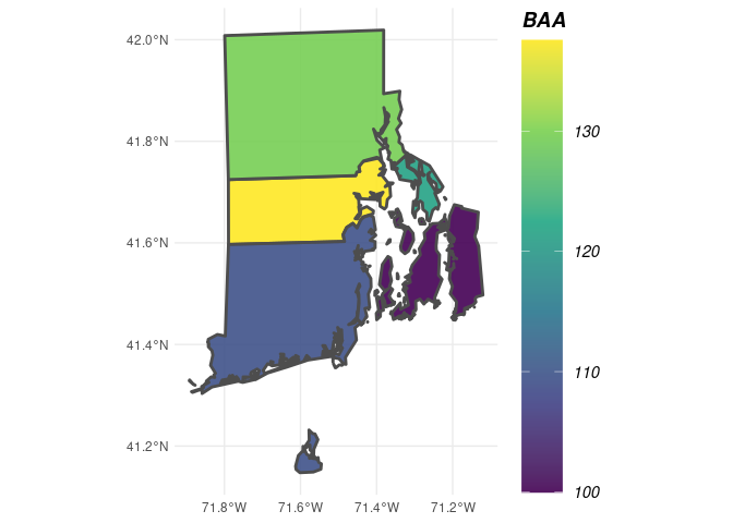
We produced a really cool time series earlier, how would I
marry the spatial and temporal capacity of rFIA to produce
estimates across user-defined polygons and through time? Easy!
Just hand tpa the full FIA.Database object you produced
with readFIA (not the most recent subset produced with
clipFIA). For stunning space-time visualizations, hand the
output of tpa to plotFIA. To save the
animation as a .gif file, simpy specify fileName (name of
output file) and savePath (directory to save file, combined
with fileName).
## Using the full FIA dataset, all available inventories
tpaRI_st <- tpa(fiaRI, polys = countiesRI, returnSpatial = TRUE)

## Animate the output
library(gganimate)
plotFIA(tpaRI_st, TPA, animate = TRUE, legend.title = 'Abundance (TPA)', legend.height = .8)
#> NULL